Decoding Loss Functions: The Unsung Hero of Machine Learning

• Introduction of Loss Function
• Popular loss functions
  • Mean Squared Error (MSE)/ Quadratic Loss/ L2 Loss:
  • Mean Absolute Error (MAE)/ L1 Loss
  • Cross-Entropy Loss/ Log Loss:
  • Hinge Loss/ Multi-class SVM Loss:
  • Huber Loss:
  • Final Plot
• Conclusion

Introduction of Loss Function

A loss function, also known as a cost function, is a method of evaluating how well a specific algorithm models the given data. If predictions deviate too much from actual results, loss function would cough up a very large number. Gradually, with the help of some optimization function, loss function learns to reduce the error in prediction. In a nutshell, the predictability of a machine learning model is directly proportional to the error rate. The less the error rate, the greater the accuracy of the model in its predictions.

Mathematically, it is represented as:

L(y, f(x))

where,

• L is the loss function,
• y is the true value, and
• f(x) is the predicted value.

Let's consider a simple example using Mean Squared Error (MSE) which is a common loss function used for regression tasks. Suppose you're trying to predict the price of a house given certain features (like the number of rooms, location, size of the house etc.). You've built a model, and for a particular house, your model predicts a price of $300,000.

Now, let's say the actual price of the house was $350,000. You can use the MSE loss function to quantify how far off your prediction was.

The MSE is calculated as the average of the squared differences between the predicted and actual values. In this case, you have only one prediction, so the MSE is simply the square of the difference between the prediction and the actual value:

MSE = (Prediction - Actual)^2
MSE = (300,000 - 350,000)^2
MSE = (-50,000)^2
MSE = 2,500,000,000

This is a very large MSE, indicating that your prediction was quite far off from the actual value.

Now, suppose you adjust your model, and now it predicts a price of $345,000 for the house. The new MSE would be:

MSE = (Prediction - Actual)^2
MSE = (345,000 - 350,000)^2
MSE = (-5,000)^2
MSE = 25,000,000

The new MSE is significantly lower, indicating that your new prediction is much closer to the actual value.

In practice, of course, you would calculate the MSE over many predictions, not just one. But this example illustrates the basic idea: the loss function gives you a measure of how far off your predictions are from the actual values, allowing you to adjust your model to try and minimize this loss.

Popular loss functions

Let's explore some of the popular loss functions in machine learning.

Mean Squared Error (MSE)/ Quadratic Loss/ L2 Loss:

Mean Squared Error (MSE) or Quadratic Loss or L2 Loss is one of the most common loss functions used in regression problems. It measures the average of the squares of the errors between the actual and the predicted values.

Mathematical Expression:

If we denote y as the vector of actual values and y_hat as the predicted values, the MSE can be calculated as follows:

MSE = (1/n) * Σ (y - y_hat)²

where n is the total number of observations.

Characteristics:

• It is differentiable, which makes it easy to compute the gradient for optimization algorithms such as Gradient Descent.
• It heavily penalizes large errors due to the squared term.
• It's sensitive to outliers due to the squaring of errors.

Application Scenarios:

MSE is widely used in various regression problems like predicting house prices, stock prices, etc. However, due to its sensitivity to outliers, it might not be the best choice when the data is prone to many outliers or extreme values.

Here is a Python code to calculate Mean Squared Error:

import numpy as np

def mse(y_true, y_pred):
    return np.mean((y_true - y_pred) ** 2)

# Test
y_true = np.array([1.0, 1.5, 2.0, 2.5, 3.0])
y_pred = np.array([1.1, 1.4, 2.1, 2.6, 3.2])

print(mse(y_true, y_pred))

Output:

0.016000000000000028

Let's also plot a graph to show how the error increases with the deviation from the true value:

import matplotlib.pyplot as plt
import numpy as np

# Deviations from the true value
x = np.linspace(-2, 2, 400)

# Calculate the MSE for each deviation
y = x ** 2

# Plot
plt.figure(figsize=(9, 6))
plt.plot(x, y, label='MSE')
plt.xlabel('Deviation from true value')
plt.ylabel('Error')
plt.legend()
plt.grid(True)
plt.title('Mean Squared Error Loss')
plt.show()

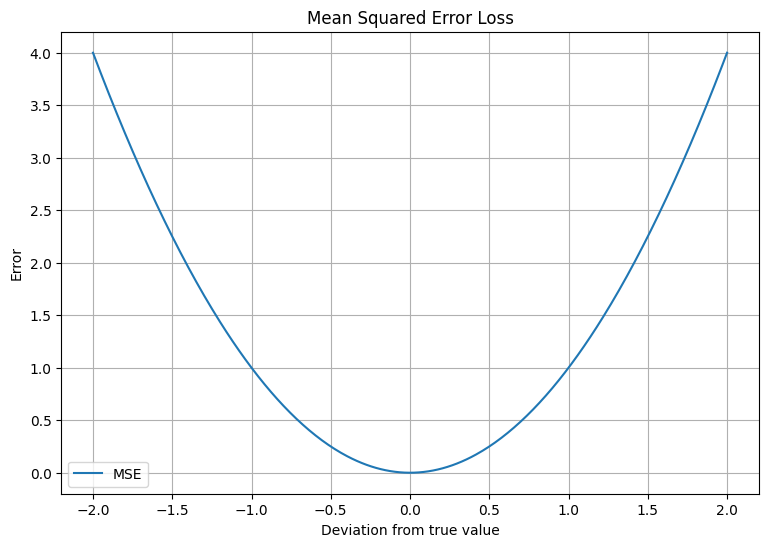
The above plot shows how the error (MSE) increases quadratically with the deviation from the true value, penalizing larger errors more heavily.

Mean Absolute Error (MAE)/ L1 Loss

Mean Absolute Error (MAE) or L1 Loss is one of the simplest regression loss functions. As its name implies, it calculates the absolute difference between the actual and predicted values, and then averages these absolute differences over the entire dataset. This makes MAE a very intuitive metric: it essentially tells you, on average, how far off your predictions are from the actual values.

Mathematically, it can be represented as follows:

MAE = (1/n) * Σ|y_true - y_pred|

Here, y_true represents the actual values, y_pred represents the predicted values, and n is the number of observations in the dataset.

MAE is less sensitive to outliers compared to the Mean Squared Error (MSE), because it does not square the differences. This means that large differences will not be disproportionately penalized, which can be useful in situations where you do not want to overreact to outliers in your data.

Application Scenarios:

MAE is commonly used in regression problems. For instance, you might use MAE when predicting house prices, temperatures, or stock prices. MAE is also often used in time series forecasting. It is best used in scenarios where the distribution of the target variable may have outliers and the effect of these outliers need to be dampened.

Python Code:

The code below defines a function for calculating Mean Absolute Error and plots the loss for predictions in the range of -3 to 3 when the actual value is 1.

import numpy as np
import matplotlib.pyplot as plt

def MAE(y_true, y_pred):
    return np.abs(y_true - y_pred)

y_true = 1
y_pred = np.linspace(-3, 3, 500)
loss = MAE(y_true, y_pred)

plt.figure(figsize=(9, 6))
plt.plot(y_pred, loss)
plt.xlabel('Predictions')
plt.ylabel('Loss')
plt.title('Mean Absolute Error Loss')
plt.grid(True)
plt.show()

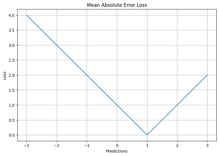
In this plot, the x-axis represents the predicted values and the y-axis represents the loss. You can see that the loss increases linearly as the prediction moves away from the true value.

Cross-Entropy Loss/ Log Loss:

Cross-Entropy Loss is commonly used in classification problems where the output of a model is a probability between 0 and 1. Cross-Entropy Loss increases as the predicted probability diverges from the actual label. So predicting a probability of 0.012 when the actual observation label is 1 would be bad and result in a high loss value.

Mathematical Expression:

The formula for a single training example's loss is:

Cross-Entropy Loss = - (y * log(y_hat) + (1 - y) * log(1 - y_hat))

where y is the actual value, and y_hat is the predicted value (probability).

Characteristics:

• It is continuously differentiable.
• It is used when the output of a model represents the probability of an outcome: It penalizes predictions that are both wrong and confident.
• It provides a steep gradient for wrong predictions, making the model learn faster.

Application Scenarios:

Cross-Entropy Loss is mainly used in binary classification problems like spam detection, tumor detection etc. It's also used in multiclass classification problems (with a slight modification to the formula).

Here's a Python code for calculating Cross-Entropy Loss:

import numpy as np

def cross_entropy(y_true, y_pred):
    return -np.sum(y_true * np.log(y_pred) + (1 - y_true) * np.log(1 - y_pred))

# Test
y_true = np.array([0, 0, 1, 1])
y_pred = np.array([0.1, 0.2, 0.7, 0.9])

print(cross_entropy(y_true, y_pred))

Outputs:

0.7905395265685948

To visualize Cross-Entropy Loss, let's plot it for a binary classification where the true label is 1:

import matplotlib.pyplot as plt

# Predicted probability
x = np.linspace(0.01, 1, 100)

# Calculate the cross-entropy loss
y = -np.log(x)

# Plot
plt.figure(figsize=(9, 6))
plt.plot(x, y, label='Cross-Entropy Loss')
plt.xlabel('Predicted Probability')
plt.ylabel('Loss')
plt.legend()
plt.grid(True)
plt.title('Cross-Entropy Loss for y=1')
plt.show()

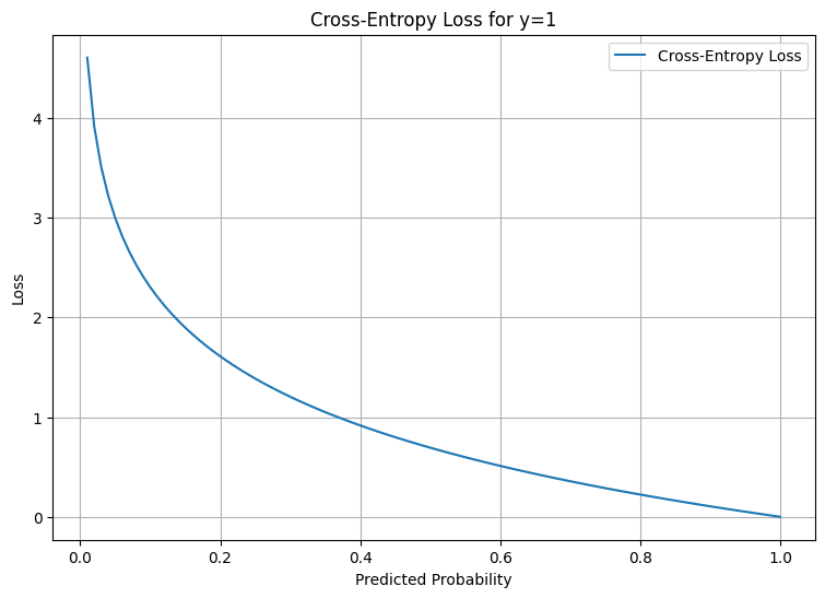
The plot shows how the loss goes to infinity as the predicted probability approaches 0, which highlights how the Cross-Entropy Loss heavily penalizes confident and wrong predictions.

Hinge Loss/ Multi-class SVM Loss:

Hinge Loss is typically used with Support Vector Machine (SVM) classifiers. The goal of an SVM classifier is to find the optimal hyperplane that separates clusters of vector in such a way that the distance from the hyperplane to the nearest vector on either side is maximized.

Mathematical Expression:

The formula for the hinge loss is:

Hinge Loss = max(0, 1 - y * y_hat)

where y is the actual value (-1 or 1 in a binary classification problem), and y_hat is the predicted value.

Characteristics:

• Hinge Loss is used for "maximum-margin" classification, most notably for Support Vector Machines (SVMs).
• Although it is intended for use with SVM, Hinge Loss can be used with other classification algorithms.
• Hinge Loss does not care about the exact values of predictions, but only their signs. Therefore, it's less sensitive to outliers than other losses like Mean Squared Error.

Application Scenarios:

Hinge Loss is mainly used in SVM for both binary and multiclass classification problems.

Here's a Python code for calculating Hinge Loss:

import numpy as np

def hinge_loss(y_true, y_pred):
    return np.maximum(0, 1 - y_true * y_pred)

# Test
y_true = np.array([-1, -1, 1, 1])
y_pred = np.array([-0.8, -0.7, 0.4, 0.6])

print(hinge_loss(y_true, y_pred))

Output:

[0.2 0.3 0.6 0.4]

To visualize Hinge Loss, let's plot it:

import matplotlib.pyplot as plt

# Predicted value
x = np.linspace(-3, 3, 100)

# Calculate the hinge loss for y=1
y = np.maximum(0, 1 - x)

# Plot
plt.figure(figsize=(9, 6))
plt.plot(x, y, label='Hinge Loss')
plt.xlabel('Predicted Value')
plt.ylabel('Loss')
plt.legend()
plt.grid(True)
plt.title('Hinge Loss')
plt.show()

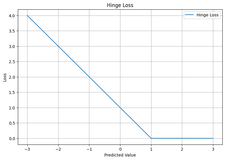
The plot shows how the loss decreases linearly as the predicted value increases from -3 to 1. Beyond 1, the loss remains 0, as the prediction is correct (the sign of the predicted value is the same as the true value).

Huber Loss:

Huber Loss, also known as Smooth Mean Absolute Error is often used in regression problems.

Mathematical Expression:

Huber Loss is less sensitive to outliers in data than mean squared error. It's defined as:

Huber Loss = 0.5*(y-y_hat)^2                  for |y-y_hat| <= delta
Huber Loss = delta * |y-y_hat| - 0.5*delta^2  otherwise

where y is the true value, y_hat is the predicted value, and delta is a hyperparameter which determines the threshold at which the loss function transitions from quadratic to linear.

Characteristics:

• Huber Loss combines the best properties of L2 squared loss and L1 absolute loss by being strongly convex when close to the target/minimum and less steep for extreme values.
• The delta value decides the cut-off point to switch from Mean Squared Error to Mean Absolute Error.
• Huber Loss is less sensitive to outliers than Mean Squared Error.

Application Scenarios:

Huber Loss is mainly used in regression problems, robust regression, and in some classification problems as well.

Here's a Python code snippet for calculating Huber Loss:

import numpy as np

def huber_loss(y_true, y_pred, delta=1.0):
    error = y_true - y_pred
    is_small_error = np.abs(error) <= delta
    squared_loss = 0.5 * error**2
    absolute_loss = delta * np.abs(error) - 0.5 * delta**2
    return np.where(is_small_error, squared_loss, absolute_loss)

# Test
y_true = np.array([1.2, 2.4, 3.6, 4.8])
y_pred = np.array([1.0, 2.2, 3.2, 4.6])

print(huber_loss(y_true, y_pred, delta=1.0))

Output:

[0.02 0.02 0.08 0.02]

To visualize Huber Loss, let's plot it:

import matplotlib.pyplot as plt

# Predicted value
x = np.linspace(-3, 3, 500)

# Calculate the Huber loss for delta=1
y = huber_loss(1, x, delta=1)

# Plot
plt.figure(figsize=(9, 6))
plt.plot(x, y, label='Huber Loss')
plt.xlabel('Predicted Value')
plt.ylabel('Loss')
plt.legend()
plt.grid(True)
plt.title('Huber Loss')
plt.show()

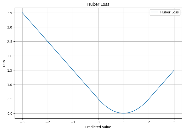
The plot shows the quadratic nature of the loss for predictions close to the true value and the linear nature of the loss for predictions far from the true value.

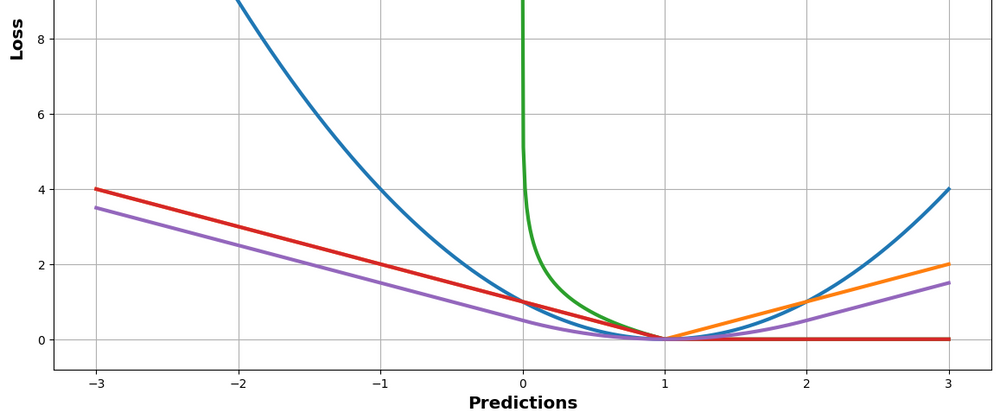
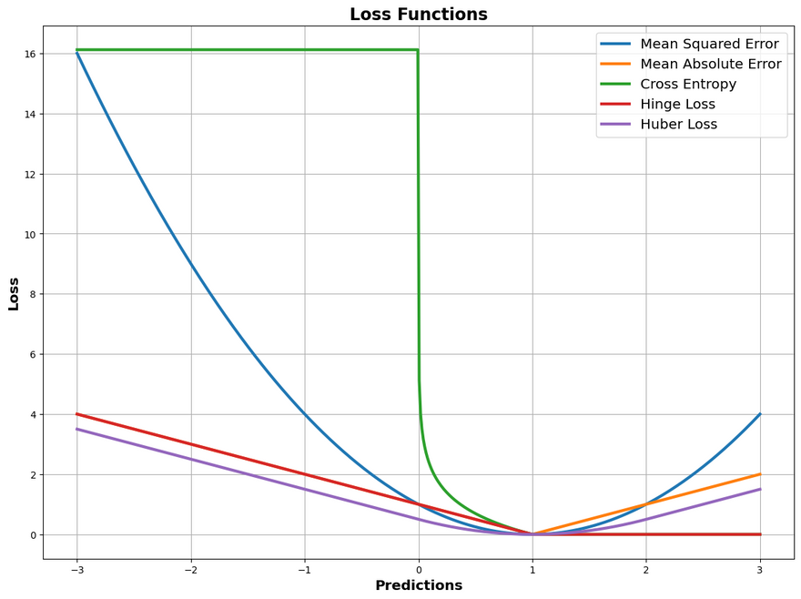
Final Plot

Lets plot all of these loss function in a same graph. Please note that the range of values and the look of the graph will vary based on the true values chosen, the range of predicted values, and the delta for the Huber loss. Adjust these as needed for your specific use case.

import numpy as np
import matplotlib.pyplot as plt

def MSE(y_true, y_pred):
    return (y_true - y_pred) ** 2

def CrossEntropy(y_true, y_pred):
    epsilon = 1e-7  # small constant to prevent log(0)
    y_pred = np.clip(y_pred, epsilon, 1 - epsilon)  # clip values to be within the range [epsilon, 1 - epsilon]
    return -(y_true * np.log(y_pred) + (1 - y_true) * np.log(1 - y_pred))

def Hinge(y_true, y_pred):
    return np.maximum(0, 1 - y_true * y_pred)

def Huber(y_true, y_pred, delta=1.0):
    return np.where(np.abs(y_true - y_pred) < delta, 0.5 * ((y_true - y_pred) ** 2), delta * (np.abs(y_true - y_pred) - 0.5 * delta))

def MAE(y_true, y_pred):
    return np.abs(y_true - y_pred)

y_true = 1
y_pred = np.linspace(-3, 3, 500)

losses = {
    "Mean Squared Error": MSE(y_true, y_pred),
    "Mean Absolute Error": MAE(y_true, y_pred),
    "Cross Entropy": CrossEntropy(y_true, y_pred),
    "Hinge Loss": Hinge(y_true, y_pred),
    "Huber Loss": Huber(y_true, y_pred)
}

plt.figure(figsize=(14, 10))
for loss_name, loss in losses.items():
    plt.plot(y_pred, loss, label=loss_name, linewidth=3)

plt.xlabel('Predictions', fontsize='x-large', fontweight='bold')
plt.ylabel('Loss', fontsize='x-large', fontweight='bold')
# plt.legend()
plt.legend(loc='best', fontsize='x-large')  # bigger font size for the legend
plt.grid(True)
plt.title('Loss Functions', fontsize='xx-large', fontweight='bold')
plt.show()

You will see output something similar to this.

Conclusion

In conclusion, loss functions are a pivotal part of any machine learning model. They provide us a way to measure how well our model is performing and to guide its learning process. Whether it's Mean Squared Error (MSE) for regression problems, Cross-Entropy Loss for classification problems, Hinge Loss for support vector machines, or the more robust Huber Loss for handling outliers, each loss function has its unique application and characteristics.

There are many other types of loss functions (such as logarithmic loss, cosine proximity, etc.), each of which has its own characteristics and application scenarios.

Choosing the right loss function is not always straightforward and depends on the specific problem and data at hand. That being said, a firm understanding of the different types of loss functions and their behavior gives us a strong foundation to make these decisions, and to customize or even develop new loss functions when necessary.

However, as with much of machine learning, it's as much an art as a science. The best way to become proficient in selecting and using loss functions is through practice, experimentation, and continuous learning. As you continue your journey in machine learning and deep learning, you'll undoubtedly encounter many opportunities to apply and further your understanding of these indispensable tools

Disclosure: Please note that the content in this blog was written with the assistance of OpenAI's ChatGPT language model.