Deep Dive - Stochastic Gradient Descent (SGD) Optimizer

• Stochastic Gradient Descent (SGD)
• Finding lost key example to explain SGD
• Feature set of SGD:
• Popular use-cases:
• Downsides:
• Stochastic Gradient Descent with different learning schedules

Stochastic Gradient Descent (SGD)

Stochastic Gradient Descent (SGD) is a variation of the gradient descent algorithm that calculates the error and updates the model for each instance in the training dataset, instead of the entire training dataset at once.

Mathematically, it can be represented as:

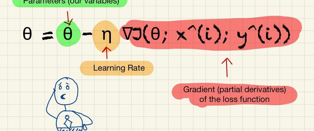
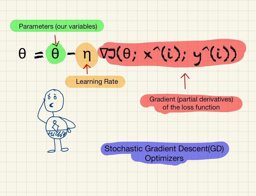
θ = θ - η ∇J(θ; x^(i); y^(i))

where:

• θ represents the parameters (or weights) of the model.
• η is the learning rate, a hyperparameter determining the step size at each iteration while moving toward a minimum of a loss function.
• ∇J(θ; x^(i); y^(i)) is the gradient (partial derivatives) of the loss function J, evaluated for the parameters θ and a single instance (x^(i), y^(i)) randomly chosen from the dataset.

In words, this formula means that for each iteration of the algorithm, we randomly select one instance (x^(i), y^(i)) from the dataset and compute the gradient of the loss function at the point specified by the current parameters θ and the instance's features x^(i) and labels y^(i). We then multiply this gradient by the learning rate η and subtract the result from the current parameters to update them.

This process is repeated for a specified number of iterations or until the parameters converge to an optimal value (i.e., the gradient is close to zero).

Finding lost key example to explain SGD

Let's use the example of trying to find a lost key in a field.

Traditional Gradient Descent is like walking blindfolded across the entire field, with each step you take being in the direction that slopes downward the most. After each step, you reassess and choose the next direction that has the steepest descent. You keep doing this until you reach a point where every direction around you is uphill, and hopefully, that's where the key is.

On the other hand, Stochastic Gradient Descent is more like a playful puppy running around in the field. Instead of calculating the steepest descent based on the entire field, the puppy simply bounds around where it is and chooses its next direction based on a small patch of grass. The puppy doesn't assess the whole field before every step. Rather, it chooses the downward direction in its immediate vicinity. This is more random and can potentially lead to finding the key faster, but also may miss the key if it only bounds around in one small area of the field.

Feature set of SGD:

• Efficiency: SGD allows us to use the same learning model with less computational resources.
• Simplicity: The algorithm is simple and easy to understand.
• Ability to escape local minima: Since the updates are noisy, this can help the algorithm escape local minima.

Popular use-cases:

SGD is useful when dealing with large-scale datasets as it's computationally much faster and efficient.

Downsides:

• Due to its stochastic (random) nature, the algorithm doesn't make steady progress towards the minimum and the error rate can bounce around. This can make the final parameters and model accuracy worse if you stop too early.
• It may take longer to achieve the global minimum than batch gradient descent because it uses a single instance, which might not be representative.
• The learning rate schedule can have a large impact on the final solution.

Let's illustrate with an example Python code:

import numpy as np
import matplotlib.pyplot as plt

# Cost function
def cost_function(x):
    return x**2

# Derivative of cost function
def derivative(x):
    return 2*x

# SGD
def sgd(x_start, epochs, learning_rate):
    x = x_start
    history = [x]
    for i in range(epochs):
        grad = derivative(x)
        x = x - learning_rate * grad
        history.append(x)
    return history

x_start = 5
epochs = 30
learning_rate = 0.9
history = sgd(x_start, epochs, learning_rate)

# Plot
plt.plot(history, [cost_function(x) for x in history], 'o-')
plt.title('SGD Optimization')
plt.xlabel('x value')
plt.ylabel('Cost function')
plt.show()

Output:

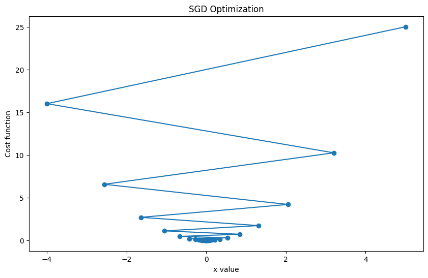
In this plot, we are showing the path taken by the SGD optimizer towards the minimum of the function x^2, starting from x=5. The optimizer successfully reaches near the minimum. The oscillations are due to the learning rate being relatively high. If the learning rate is decreased, the path would be smoother.

Stochastic Gradient Descent with different learning schedules

Let's use a simple linear regression problem and solve it using Stochastic Gradient Descent (SGD) with different learning rates and iteration counts.

import numpy as np
import matplotlib.pyplot as plt

# Let's create a simple linear regression problem.
np.random.seed(0)
X = 2 * np.random.rand(100,1)
y = 4 + 3 * X + np.random.randn(100,1)

# SGD requires feature scaling. Here we do manual scaling.
X_b = np.c_[np.ones((100,1)), X]
X_b = X_b / np.linalg.norm(X_b, axis=0)

# Our SGD implementation
def SGD(X_b, y, lr_schedule, m_init, b_init, num_epochs):
    m = m_init
    b = b_init
    m_list, b_list, epoch_list, mse_list = [], [], [], []

    for epoch in range(num_epochs):
        for i in range(X_b.shape[0]):
            random_index = np.random.randint(X_b.shape[0])
            xi = X_b[random_index:random_index+1]
            yi = y[random_index:random_index+1]

            gradients = 2 * xi.T.dot(xi.dot(np.array([b, m]).T) - yi)
            eta = lr_schedule(epoch * X_b.shape[0] + i)
            b, m = np.array([b, m]).T - eta * gradients

        y_pred = X_b.dot(np.array([b, m]).T)
        mse = np.mean((y - y_pred)**2)
        m_list.append(m[0])
        b_list.append(b[0])
        epoch_list.append(epoch)
        mse_list.append(mse)
    return m_list, b_list, epoch_list, mse_list

# Let's use SGD with three different learning schedules
np.random.seed(42)
m_init = np.random.randn()
b_init = np.random.randn()

# Learning schedule 1: Constant learning rate
lr_schedule_1 = lambda x: 0.01
m1, b1, epochs1, mse1 = SGD(X_b, y, lr_schedule_1, m_init, b_init, num_epochs=50)

# Learning schedule 2: Learning rate decays over time
lr_schedule_2 = lambda x: 0.01 * np.exp(-x/50)
m2, b2, epochs2, mse2 = SGD(X_b, y, lr_schedule_2, m_init, b_init, num_epochs=50)

# Learning schedule 3: Learning rate oscillates
lr_schedule_3 = lambda x: 0.01 * (np.cos(x/50) + 1)/2
m3, b3, epochs3, mse3 = SGD(X_b, y, lr_schedule_3, m_init, b_init, num_epochs=50)

# Now, let's plot the learning curves for all three learning schedules
plt.figure(figsize=(12,8))

plt.plot(epochs1, mse1, label='Constant learning rate', linewidth=2)
plt.plot(epochs2, mse2, label='Decaying learning rate', linewidth=2)
plt.plot(epochs3, mse3, label='Oscillating learning rate', linewidth=2)

plt.xlabel('Epoch', fontsize=14)
plt.ylabel('Mean Squared Error', fontsize=14)
plt.title('Stochastic Gradient Descent with different learning schedules', fontsize=16)
plt.legend()
plt.grid(True)
plt.show()

Output:

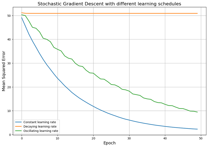
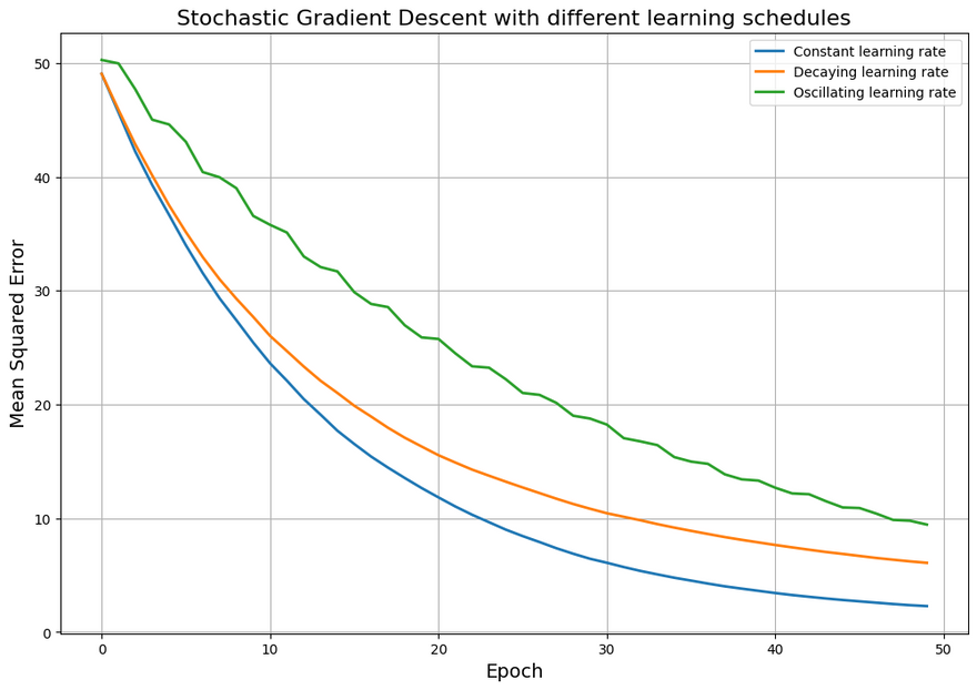
In this plot, you can see how,

• Constant learning rate: The error reduces consistently with each epoch. This suggests that the model is continually learning and the error is decreasing as the model becomes more accurate.

• Decaying learning rate: The error reduces slightly in the initial epochs, but then becomes steady. This could suggest that the learning rate has decayed too much and the model has stopped learning before reaching its maximum potential or the minimum loss.

  When using a decaying learning rate, the idea is to start with a large learning rate to make big changes in the model parameters initially, then reduce the learning rate over time to make smaller and more precise updates. However, if the learning rate decays too quickly or too much, it can become so small that the updates to the model parameters are negligible. This means that the model stops learning effectively and the error stops decreasing, leading to the constant error value you're seeing.

  One way to address this issue could be to use a slower decay rate or to set a lower bound on the learning rate to ensure it never becomes too small. These adjustments would prevent the learning rate from reaching a value that hampers the learning process while still taking advantage of the benefits of a decaying learning rate. For example we can adjust slower decay rate as follows in above code base,
  

  # Learning schedule 2: Learning rate decays over time
  lr_schedule_2 = lambda x: 0.01 * np.exp(-x/5000)
  m2, b2, epochs2, mse2 = SGD(X_b, y, lr_schedule_2, m_init, b_init, num_epochs=50)
  

  Which will produce following output,

  

• Oscillating learning rate (epochs3): The error decreases overall but not smoothly, reflecting the oscillations in the learning rate. These oscillations could cause slower convergence or might lead to instability if they are too large.

Disclosure: Please note that the content in this blog was written with the assistance of OpenAI's ChatGPT language model.