Deep Dive - Gradient Descent (GD) Optimizer

• Gradient Descent (GD)
  • Hiking Example to explain Gradient Descent
  • Amusement Park Example
  • Features of GD:
  • Popular Use Cases:
  • Downside:
  • Effect of Learning Rate on Gradient Descent
  • Gradient Descent getting stuck in local minima

Disclosure: Please note that the content in this blog was written with the assistance of OpenAI's ChatGPT language model.

Gradient Descent (GD)

Gradient Descent (GD) is a first-order iterative optimization algorithm for finding a local minimum of a differentiable function. The idea of Gradient Descent is to tweak parameters iteratively in order to minimize a cost function.

The mathematical notation for the update rule of GD is given by:

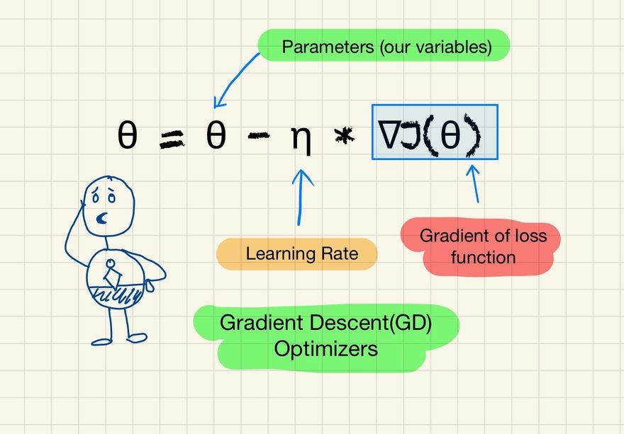
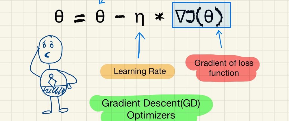
θ = θ - η * ∇J(θ)

Here:

• θ represents the parameters (our variables)
• η is the learning rate (how fast we want to learn)
• ∇J(θ) is the gradient of the loss function.

Hiking Example to explain Gradient Descent

This is a lot of information, let's try to explain Gradient Descent in simpler example using a popular example in this space.

Imagine you're hiking on a mountain range, and your goal is to get to the lowest point in the valley. It's a foggy day, and you can't see very far ahead. So, what do you do? You might look around and see which way the ground slopes down the most and take a step in that direction.

This is essentially what Gradient Descent does. It measures the local gradient of the error function with regards to the parameter vector, and it goes in the direction of descending gradient. Once the gradient is zero, you have reached a minimum!

If the ground slopes downward to your left, you would take a step to the left. If it slopes downward to your right, you'd step right. You'd keep doing this until you reach a point where the ground doesn't slope down in any direction - you've reached the lowest point you can get to. In technical terms, you've reached a local minimum of the function.

An important part of this analogy is that the size of your steps matters. If your steps are too small, it could take a long time to get to the bottom. If your steps are too large, you might overshoot the bottom and end up on the other side of the valley, or even higher up on the mountain. This step size is referred to as the learning rate in Gradient Descent.

So in simple terms, Gradient Descent is like a hiker (the model) trying to get to the bottom of a valley (the minimum of the cost function), who can only see a small part of the mountain (the local gradient of the cost function) and takes steps that are too small or too large could make the hike longer or even impossible (the learning rate).

Amusement Park Example

Let's consider a different example.

Imagine you're at a giant amusement park and you've heard that there's a specific amazing ride you must experience. The problem is, you don't have a map of the park and it's a particularly busy day so you can't see the entire park from where you are standing due to the crowd. Your goal is to find this ride as quickly as possible.

You notice signboards across the park that give you the direction and distance to the nearest attractions. Now, you could potentially check out all attractions hoping to find the ride but that would be too time-consuming.

So, you decide to ask people coming from different directions about the ride. Based on their responses, you gauge which direction you should head to next.

Every time you choose a direction, you're essentially making a 'guess' and correcting it based on the feedback you get from the people you ask. Over time, these little corrections will hopefully guide you towards the desired ride.

This scenario is similar to what happens in gradient descent. Your location in the park represents the parameters of the model, the feedback you get is equivalent to the gradient of the loss function, and your goal (the ride) is the minimum of the loss function. The people's guidance you use to correct your course is the step taken in the direction of the steepest descent (the negative gradient).

In this process, the 'size' of the steps you take is the learning rate. If you take small steps (low learning rate), it may take you a longer time to reach the ride but you would be sure about every step. If you take larger steps (high learning rate), you might reach faster, but there's also a chance you could bypass the ride without noticing it.

Just like in the amusement park scenario, gradient descent uses feedback (calculating the gradient) to correct its 'guesses' (parameters of the model) and iteratively refines these guesses until it finds the best possible answer (minimum of the loss function).

Features of GD:

• Simplicity: Gradient Descent is simple and easy to implement.
• Scalability: GD scales to problems with many parameters efficiently.

Popular Use Cases:

Gradient Descent forms the basis of many machine learning algorithms and is used in neural networks, linear regression, Support Vector Machines (SVMs), etc.

Downside:

• Choosing a proper learning rate can be difficult. A learning rate that is too small leads to painfully slow convergence, while a learning rate that is too large can hinder convergence and cause the loss function to fluctuate around the minimum or even to diverge.
• Gradient Descent can get stuck in shallow local minima in case of non-convex error surfaces.

Here is a simple example illustrating the concept of Gradient Descent using Python:

import numpy as np
import matplotlib.pyplot as plt

# Our function to optimize (loss function)
def func(x):
    return x**2 + x*4 + 9

# Derivative of the function (gradient)
def gradient(x):
    return 2*x + 4

# Gradient descent
def gradient_descent(start_at=np.random.uniform(-10, 10), 
                     learn_rate=0.1, 
                     n_iter=50):
    x = start_at
    trajectory = [x]

    for i in range(n_iter):
        grad = gradient(x)
        x = x - learn_rate * grad
        trajectory.append(x)

    return np.array(trajectory)

# Plotting
trajectory = gradient_descent()

plt.figure(figsize=(10, 5))
x = np.linspace(-15, 10, 400)
y = func(x)

plt.plot(x, y, label="Loss Function")
plt.plot(trajectory, func(trajectory), '-o', color="red", label="Gradient Descent")
plt.title('Gradient Descent Optimization')
plt.xlabel('x')
plt.ylabel('f(x)')
plt.legend()
plt.grid()
plt.show()

Output:

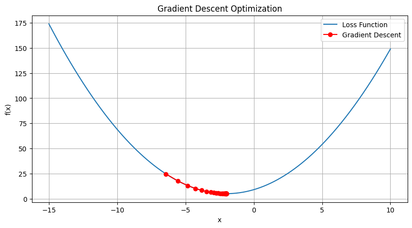
In this Python code, we define a simple quadratic function and its gradient. We implement gradient descent, starting from a random point. The 'learning_rate' parameter controls how large a step we take downhill during each iteration. 'n_iter' is the number of steps we'll take. We save our position at each step in 'trajectory', which we can then plot. The red dots in the plot represent the steps of gradient descent.

Please note that the learning rate and the number of iterations are hyperparameters - you can adjust them to see how they affect the algorithm.

Effect of Learning Rate on Gradient Descent

To explain the effect of learning rate on the convergence of Gradient Descent, we need to simulate gradient descent under different learning rates.

Here's a simple python code to illustrate this. We will use a simple quadratic function as our loss function for simplicity.

import numpy as np
import matplotlib.pyplot as plt

def gradient_descent(learning_rate, iterations):
    x = 3 # starting point
    results = [x]
    for i in range(iterations):
        grad = 2*x  # derivative of x^2
        x = x - learning_rate * grad
        results.append(x)
    return results

# parameters
iterations = 10

# learning rates
rates = [0.01, 0.1, 0.9, 1.1]

# plot the descent for different learning rates
plt.figure(figsize=(12, 8))

for rate in rates:
    results = gradient_descent(rate, iterations)
    plt.plot(range(iterations+1), results, label=f'learning rate: {rate}')

plt.legend()
plt.xlabel('Iteration')
plt.ylabel('x value')
plt.title('Effect of learning rate on Gradient Descent')
plt.grid(True)
plt.show()

Output:

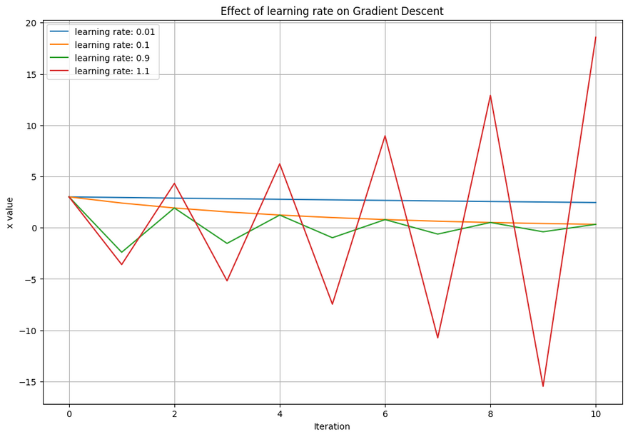
In this plot, you can observe the effect of learning rate on the convergence of gradient descent. A small learning rate (like 0.01) makes the descent slow and steady, while a larger learning rate (like 0.1) speeds it up. However, a too large learning rate (like 0.9 or 1.1) causes overshooting, where it bounces back and forth across the minimum, or diverges entirely.

Gradient Descent getting stuck in local minima

To illustrate the second downside of Gradient Descent - getting stuck in local minima - we need to use a non-convex function.

Let's take a function like f(x) = x*cos(x) which has several local minima. We will initialize our gradient descent at two points and see how it converges to different minima based on the initialization.

Here is a Python code that demonstrates this:

import numpy as np
import matplotlib.pyplot as plt

# our non-convex function
def func(x):
    return x * np.cos(x)

# derivative of our function
def grad_func(x):
    return np.cos(x) - x * np.sin(x)

# simple gradient descent implementation
def gradient_descent(start_at, learning_rate, iterations):
    x = start_at
    results = [x]
    for i in range(iterations):
        x = x - learning_rate * grad_func(x)
        results.append(x)
    return results

# parameters
iterations = 50
learning_rate = 0.1

# initialization points
starts = [-2, 1]

# plot the function
x = np.linspace(-10, 10, 400)
y = func(x)

plt.figure(figsize=(10, 6))
plt.plot(x, y)

# plot the descent from different starting points
for start in starts:
    results = gradient_descent(start, learning_rate, iterations)
    y_results = func(np.array(results))
    plt.scatter(results, y_results, label=f'start at: {start}')

plt.legend()
plt.title('Gradient Descent getting stuck in different local minima')
plt.xlabel('x')
plt.ylabel('f(x)')
plt.grid(True)
plt.show()

Output:

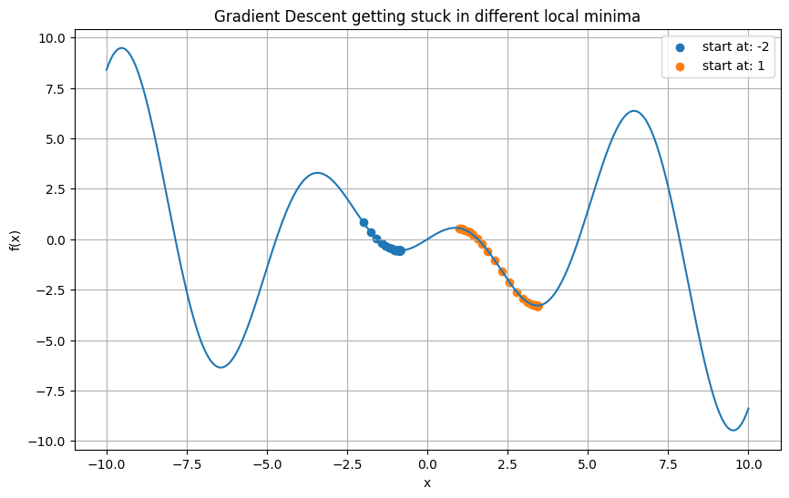
In this plot, you can observe how Gradient Descent starting from different points converges to different local minima. This is due to the non-convexity of the function, causing the Gradient Descent to get "stuck" in the closest local minima.