How Do Neural Networks Make Decisions? A Look at Activation Functions

• What is Activation function?
• Why Activation function?
• Why we need to introduce non-linearity?
• How activation function works?
• Some commonly used activation function
  • Sigmoid Function:
  • Tanh Function (Hyperbolic Tangent):
  • ReLU (Rectified Linear Unit):
  • Leaky ReLU:
  • Softmax Function:
  • Swish:
• Bonus: Comparing all activation functions.

Disclosure: Please note that the content in this blog was written with the assistance of OpenAI's ChatGPT language model.

What is Activation function?

An activation function in a neural network is a mathematical function that is applied to a neuron's output (or, in terms of the mathematics of neural networks, the activation). The purpose of the activation function is to introduce non-linearity into the network, which allows it to learn complex patterns. Without an activation function, no matter how many layers your network has, it would still behave just like a single-layer model, because the composition of linear functions is still a linear function.

If we define activation function in a simple terms, an activation function in a neural network is like the decision-making part of a neuron. Imagine a neuron in the brain that receives different kinds of information. It needs to decide whether the information it's receiving is important enough to pass along or not. That's essentially what an activation function does.

When a neural network is learning from data, it's adjusting its own internal values based on the input it receives (like pictures, text, or numbers). The activation function helps the network use these values to make decisions by answering the question, "Is the input I received important, and how important is it?"

Why Activation function?

The reason why we need activation functions is because they allow the neural network to learn from more complex data. Without activation functions, the neural network would only be able to make decisions based on a straightforward calculation from its input data. With an activation function, the neural network can learn complex patterns and make decisions that are not just straightforward calculations, but involve more subtle patterns in the data.

For example, in a network that's learning to identify dogs in pictures, an activation function might help the network learn not just to identify a dog based on its shape, but also to identify subtler patterns, like the texture of its fur or the shape of its eyes. This helps the network make better, more accurate decisions.

Why we need to introduce non-linearity?

Introducing non-linearity into machine learning models, specifically neural networks, allows the model to capture complex patterns and relationships in the data. This is particularly important when dealing with real-world data, where relationships between variables are often non-linear.

If we only use linear transformations, no matter how many layers our neural network has, it will still behave like a single-layer network. This is because the composition of linear functions is still a linear function. For example, if f(x) = 2x and g(x) = 3x, then the composition of f and g is (f ∘ g)(x) = f(g(x)) = f(3x) = 2 * 3x = 6x, which is still a linear function.

On the other hand, by introducing non-linear activation functions, each layer of the network is able to capture different transformations of the input data, which makes the model more powerful and flexible. It allows the model to learn complex decision boundaries and makes it possible to approximate virtually any continuous function, given a sufficient number of neurons and layers.

Without non-linearities, our neural network would be much less powerful and wouldn't be able to model complex data as effectively.

Let's say you are designing a spam detection system that classifies emails as either "spam" or "not spam". Each email is represented by a set of features, such as the frequency of certain words, the length of the email, the sender's email address, etc.

A linear model would classify an email as spam or not based solely on a linear combination of these features. This means that it would essentially draw a straight line (or a plane, or a hyperplane in higher dimensions) to separate the spam emails from the non-spam emails in the feature space. Any email that falls on one side of the line would be classified as spam, and any email that falls on the other side would be classified as not spam.

However, the relationship between the features of an email and whether it's spam or not is likely not linear. For example, a certain combination of words might be indicative of spam, but only if the email is also from an unknown sender. A linear model wouldn't be able to capture this kind of relationship.

Now let's add a non-linear activation function to our model. This would allow our model to learn non-linear decision boundaries, or in other words, non-linear relationships between the features and the target variable (spam or not spam).

This means that our model could learn to classify an email as spam if it contains certain words AND is from an unknown sender. This kind of complex decision-making is enabled by the non-linear activation function.

How activation function works?

An activation function in a neural network defines how the weighted sum of the input is transformed into an output from a neuron's node. It takes in the output signal from the previous cell and converts it into some form that can be taken as input for the next layer. This is called "firing" or "activating" the neuron.

Here's a simplified way of how it works:

• Linear Transformation: Each input to a neuron is multiplied by a weight. All of the weighted inputs are then added together with a bias term. This is a linear transformation of the input. Mathematically, this can be represented as z = w1*x1 + w2*x2 + ... + wn*xn + b, where w1, w2, ..., wn are weights, x1, x2, ..., xn are inputs, b is the bias, and z is the linear transformation of the inputs.

• Activation Function: This output z is then passed through an activation function f. The purpose of the activation function is to introduce non-linearity into the output of a neuron. This transformed output f(z) is then sent as input to the next layer in the network.

So, if we have an activation function f, the output y of the neuron is y = f(z).

Different activation functions will transform the input signals in different ways. For example, a sigmoid activation function will squash the input values between 0 and 1, a ReLU (Rectified Linear Unit) activation function will set all negative inputs to 0, and a tanh activation function will squash input values between -1 and 1. These transformations allow the neural network to learn complex patterns and relationships in the input data.

Some commonly used activation function

There are several commonly used activation functions in neural networks:

Sigmoid Function:

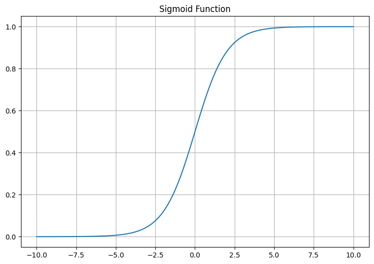
The sigmoid function takes a real-valued number and squashes it into range between 0 and 1. It's often used in the output layer of a binary classification model where the model predicts the probability of input belonging to a certain class.

• Mathematical Expression of Sigmoid Function: The function is given by the formula:

f(x) = 1 / (1 + e^-x)

Where e is the base of the natural logarithm, and x is the input to the function.

• Real-life application of Sigmoid Function:

The sigmoid function is commonly used in binary classification problems in machine learning. For instance, let's say you have a spam detection model that reads your emails and decides whether an email is spam (1) or not spam (0). The sigmoid function is used in the output layer of the neural network to squash output values between 0 and 1, which can be interpreted as the probability of the email being spam.

• Mathematical Example:

Let's calculate the sigmoid of a few values:

• For x=0, sigmoid(x) is 0.5.
• For x=1, sigmoid(x) is approximately 0.73.
• For x=-1, sigmoid(x) is approximately 0.27.

Notice how all values are between 0 and 1.

For example, Let's calculate sigmoid(1) as follows,

• Calculate e^-1. Using a calculator or a software tool, you'll find that e^-1 is approximately 0.36788.
• Plug this value into the formula:

sigmoid(1) = 1 / (1 + 0.36788)
= 1 / 1.36788
= 0.731058

• Python Code to Illustrate Sigmoid Function:

Here is a simple Python code to illustrate the sigmoid function:

import numpy as np
import matplotlib.pyplot as plt

def sigmoid(x):
    return 1 / (1 + np.exp(-x))

# generate a range of numbers between -10 and 10
x = np.linspace(-10, 10, 100)

# apply the sigmoid function to these numbers
y = sigmoid(x)

plt.figure(figsize=(9, 6))
plt.plot(x, y)
plt.title("Sigmoid Function")
plt.grid(True)
plt.show()

This code generates a range of numbers between -10 and 10 and applies the sigmoid function to these numbers. It then plots the result, showing how the sigmoid function squashes the input values into the range between 0 and 1.

Output:

Tanh Function (Hyperbolic Tangent):

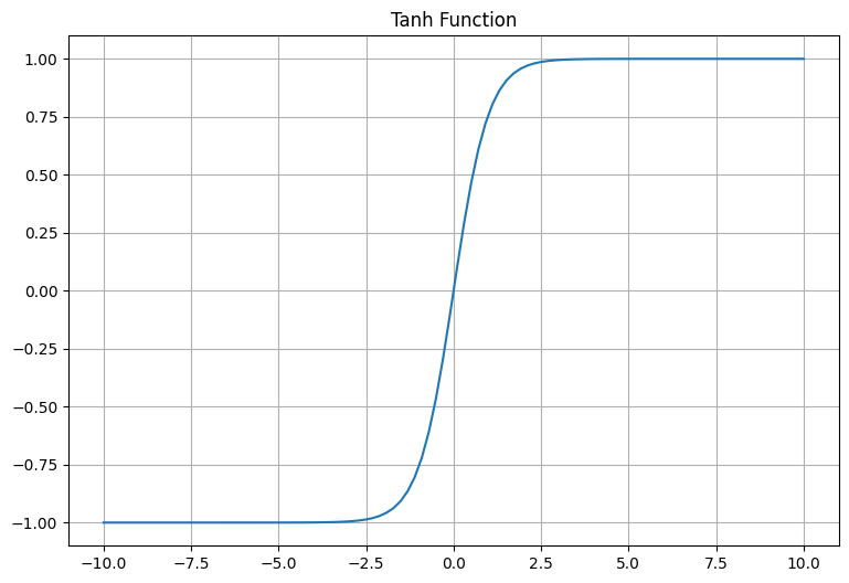
The tanh function also takes a real-valued number and squashes it into the range between -1 and 1. It's like a rescaled version of the sigmoid function and is often preferred over the sigmoid function in hidden layers of a neural network because it leads to zero-centered outputs.

• Mathematical Expression of Tanh Function: The function is given by the formula:

f(x) = (e^x - e^-x) / (e^x + e^-x)

Where e is the base of the natural logarithm, and x is the input to the function. This function outputs values in the range between -1 and 1.

• Real-life application of Tanh Function:

Just like the sigmoid function, the tanh function is also used as an activation function in neural networks. For instance, in recurrent neural networks (RNNs) used for tasks like language translation or speech recognition, the tanh function is often used to control the activations or "state" of the network over time.

• Mathematical Example:

Let's calculate the tanh of a few values:

• For x=0, tanh(x) is 0.
• For x=1, tanh(x) is approximately 0.76.
• For x=-1, tanh(x) is approximately -0.76. Notice how all values are between -1 and 1.

For example, let's calculate tanh(1):

• Calculate e^1 and e^-1. Using a calculator or a software tool, you'll find that e^1 is approximately 2.71828, and e^-1 is approximately 0.36788.

• Plug these values into the formula:
  

tanh(1) = (2.71828 - 0.36788) / (2.71828 + 0.36788)
= 2.3504 / 3.08616
= 0.761594

So tanh(1) is approximately 0.761594.

Please note, you might find slight differences in the calculated result due to the precision of the e value used in the calculation. The value of e is actually an irrational number, so its decimal representation goes on forever without repeating.

• Python Code to Illustrate Tanh Function: Here is a simple Python code to illustrate the tanh function:

import numpy as np
import matplotlib.pyplot as plt

def tanh(x):
    return np.tanh(x)

# generate a range of numbers between -10 and 10
x = np.linspace(-10, 10, 100)

# apply the tanh function to these numbers
y = tanh(x)

plt.figure(figsize=(9, 6))
plt.plot(x, y)
plt.title("Tanh Function")
plt.grid(True)
plt.show()

This code generates a range of numbers between -10 and 10 and applies the tanh function to these numbers. It then plots the result, showing how the tanh function squashes the input values into the range between -1 and 1.

Output:

ReLU (Rectified Linear Unit):

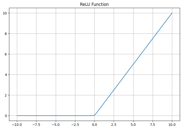
The ReLU function takes a real-valued number and thresholds it at zero (replaces negative values with zero). It has become very popular in recent years because it helps to alleviate the vanishing gradient problem, which is a difficulty found in training neural networks with gradient-based learning methods and backpropagation.

• Mathematical Expression of ReLU Function: The function returns 0 if the input is negative, and the input itself if the input is equal to or greater than 0. This can be represented mathematically as follows:

f(x) = max(0, x)

• Real-life application of ReLU Function:
  ReLU is a very popular choice for an activation function in various deep learning models and convolutional neural networks (CNNs). It is used in tasks like image and speech recognition, natural language processing, and many other machine learning tasks. The use of ReLU helps to mitigate the vanishing gradient problem, which is a common issue during the training of deep neural networks.

• Mathematical Example:

Let's calculate ReLU(-1), where x is -1:

ReLU(-1) = max(0, -1)
         = 0

So ReLU(-1) is 0.

Now, let's calculate ReLU(0), where x is 0:

ReLU(0) = max(0, 0)
        = 0

So ReLU(0) is also 0.

Lastly, let's calculate ReLU(1), where x is 1:

ReLU(1) = max(0, 1)
        = 1

So ReLU(1) is 1.

As you can see, if the input is less than or equal to zero, the output is zero. If the input is greater than zero, the output is the same as the input.

• Python Code to Illustrate ReLU Function:

Here is a simple Python code to illustrate the ReLU function:

import numpy as np
import matplotlib.pyplot as plt

def relu(x):
    return np.maximum(0, x)

# generate a range of numbers between -10 and 10
x = np.linspace(-10, 10, 100)

# apply the ReLU function to these numbers
y = relu(x)

plt.figure(figsize=(9, 6))
plt.plot(x, y)
plt.title("ReLU Function")
plt.grid(True)
plt.show()

This code generates a range of numbers between -10 and 10 and applies the ReLU function to these numbers. It then plots the result, showing how the ReLU function squashes the input values to the range between 0 and the input if the input is greater than 0.

Output:

Leaky ReLU:

Leaky ReLU is a variant of ReLU that allows small negative values when the input is less than zero. This small slope ensures that Leaky ReLU never dies and can keep learning if it enters a region of negative input space.

• Mathematical Expression: Leaky ReLU function is defined mathematically as:

f(x) = x, for x > 0
f(x) = αx, for x ≤ 0

where α is a small constant. Unlike the standard ReLU function, Leaky ReLU allows the pass of a small gradient signal for negative values. Hence, it has the advantage of allowing gradients to flow through the architecture to the weights.

• Real Life Application:
  Leaky ReLU is widely used in deep learning applications. It's commonly used in Convolutional Neural Networks (CNNs) and other types of Neural Networks where the standard ReLU function can cause a problem called "dead neurons," in which neurons essentially become inactive and no longer contribute any information to the model.

• Mathematical Example:

Let's use α = 0.01 as a commonly used value.
For x = 5, f(5) = 5 (because 5 > 0)
For x = -5, f(-5) = 0.01 * -5 = -0.05 (because -5 < 0)

• Python Code to Illustrate Leaky ReLU Function:

import numpy as np
import matplotlib.pyplot as plt

def leaky_relu(x, alpha=0.1):
    return np.maximum(alpha * x, x)

# Generate a range of values from -10 to 10
x = np.linspace(-10, 10, 1000)

# Apply the leaky ReLU function
y = leaky_relu(x)

# Create the plot
plt.figure(figsize=(9, 6))
plt.plot(x, y)
plt.title("Leaky ReLU Activation Function")
plt.xlabel("Input Value")
plt.ylabel("Output Value")
plt.grid(True)
plt.show()

This code will generate a plot showing the Leaky ReLU function. For positive input values, the output is equal to the input (a straight line). For negative input values, the output is a small, non-zero value, determined by the alpha parameter. The alpha parameter in this case is set to 0.1, but you can change this value to see how it affects the shape of the function.

Output:

Softmax Function:

The Softmax function, also known as the normalized exponential function, is used when we have a multiclass classification problem. It takes a vector of 'n' real numbers and normalizes it into a probability distribution consisting of 'n' probabilities proportional to the exponentials of the input numbers. The mathematical formula for softmax is:

S(y_i) = e^(y_i) / Σ e^(y_j)

where j goes from 1 to n.

• Real Life Application:

Softmax is mainly used in machine learning algorithms for multi-class classification, where the goal is to classify instances into one of several possible classes. For instance, it could be used to classify emails into different categories, recognize handwriting, or identify the species of a flower based on certain measurements.

• Mathematical Example:

Suppose we have a vector [1, 2, 3] and we want to compute the softmax of this vector.

First, we calculate the exponential of each element:

e^(1) = 2.71828
e^(2) = 7.38906
e^(3) = 20.0855

Next, we calculate the sum of these values:

Σ e^(y_j) = 2.71828 + 7.38906 + 20.0855 = 30.1928

Finally, we divide each element's exponential by this sum:

S(1) = e^(1) / Σ e^(y_j) = 2.71828 / 30.1928 = 0.090
S(2) = e^(2) / Σ e^(y_j) = 7.38906 / 30.1928 = 0.245
S(3) = e^(3) / Σ e^(y_j) = 20.0855 / 30.1928 = 0.665

So, the softmax of [1, 2, 3] is [0.090, 0.245, 0.665]. The values sum to 1, which makes them interpretable as probabilities.

• Python Code:

Here's how to compute the softmax function in Python:

import numpy as np
import matplotlib.pyplot as plt

def softmax(x):
    e_x = np.exp(x - np.max(x)) # subtract max(x) for numerical stability
    return e_x / e_x.sum()

# test with a vector
x = np.array([1, 2, 3])
y = softmax(x)
print(softmax(x))

# Create the bar plot
plt.figure(figsize=(6, 4))
plt.bar(range(len(x)), y)
plt.xlabel('Class')
plt.ylabel('Probability')
plt.title('Softmax output for input [1, 2, 3]')
plt.xticks(range(len(x)), ['Class 1', 'Class 2', 'Class 3'])
plt.show()

Output:

[0.09003057 0.24472847 0.66524096]

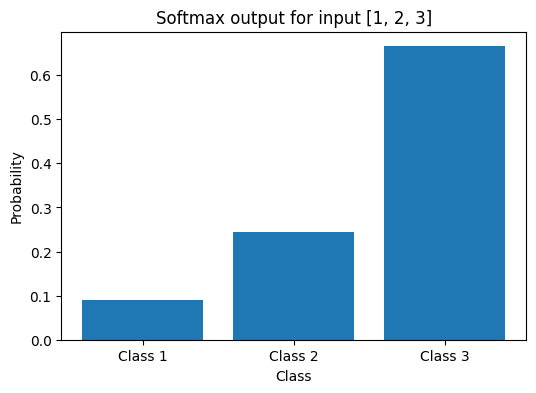
The returned array represents the probabilities of the input values, and the sum of all the values is 1, as expected.

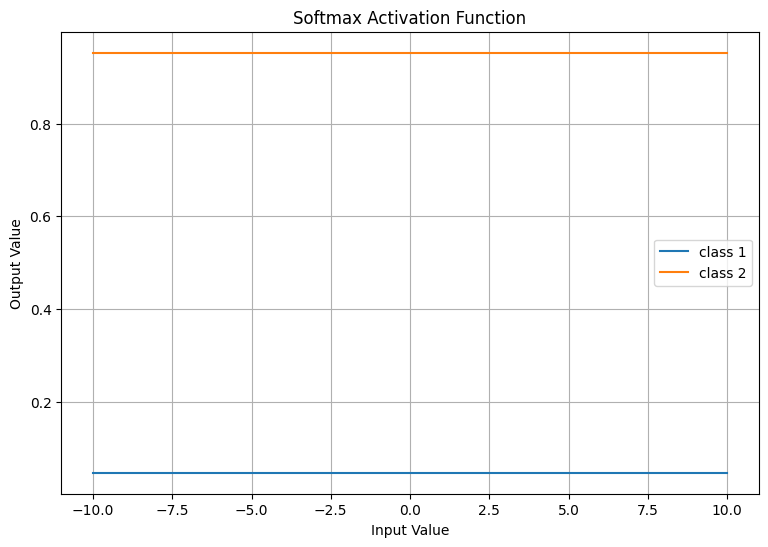
The softmax function is typically used for multiclass classification problems at the output layer of a neural network, not as an activation function in the hidden layers like ReLU or Leaky ReLU.

In the case of softmax, it expects a vector of raw scores (logits) and converts them into probabilities, such that the sum of the probabilities equals 1. This makes it suitable for multiclass classification where we want a probability distribution over multiple classes.

In contrast, ReLU or Leaky ReLU are functions applied elementwise, meaning they operate independently on each element of the input tensor.

Because of these differences, visualizing the softmax function like we did with ReLU or Leaky ReLU isn't exactly applicable. In the case of ReLU and Leaky ReLU, we visualized how an individual input value gets transformed by the function, whereas softmax considers all elements in the input vector in order to compute the probabilities.

However, if you want to visualize the softmax values for a series of input values, you can do something like this:

import numpy as np
import matplotlib.pyplot as plt

def softmax(x):
    e_x = np.exp(x - np.max(x)) # subtract max(x) for numerical stability
    return e_x / e_x.sum(axis=0)

# Generate a range of values from -10 to 10
x1 = np.linspace(-10, 10, 1000)
x2 = x1 + 3 # Shift the scores for the second class upwards
x = np.vstack([x1, x2]) # softmax expects a vector of scores for each class

# Apply the softmax function
y = softmax(x)

# Create the plot
plt.figure(figsize=(9, 6))
plt.plot(x[0], y[0], label='class 1')
plt.plot(x[0], y[1], label='class 2')
plt.title("Softmax Activation Function")
plt.xlabel("Input Value")
plt.ylabel("Output Value")
plt.grid(True)
plt.legend()
plt.show()

Output:

In this plot, you can see how the softmax function assigns a higher probability to the class with the higher score (in this case, class 2). As the score for class 1 increases, its probability also increases, but once it's less than the score for class 2, the softmax function assigns it a lower probability. This is the property of the softmax function that makes it useful for multi-class classification problems.

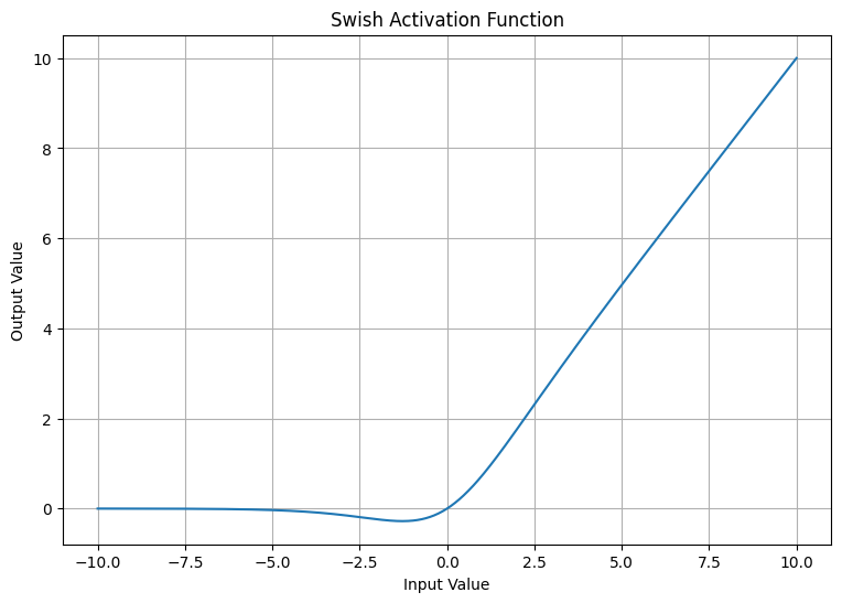
Swish:

Swish is a relatively newer activation function introduced in the paper "Searching for Activation Functions" by Google. It's a smooth, non-monotonic function that tends to work better than ReLU on deeper models across a number of challenging datasets.

It's defined as:

f(x) = x * sigmoid(x)

where sigmoid(x) = 1 / (1 + exp(-x)). So, you can see it as a combination of both the linear and sigmoid function.

Swish tends to work better in practice than ReLU on deeper models across a number of challenging data sets. For example, it has been used in tasks like image classification, where deep learning models with many layers are used.

• Mathematical calculation: Let's calculate the Swish activation for the input value x=2.

f(x) = x * sigmoid(x)
= 2 * sigmoid(2)
= 2 * 1 / (1 + exp(-2))
= 2 * 1 / (1 + 0.135)
= 2 * 0.88
= 1.76

So, the output of the Swish function for x=2 is approximately 1.76.

• Python code for the Swish function:

Here's a simple Python function for Swish and a plot to visualize it:

import numpy as np
import matplotlib.pyplot as plt

def swish(x):
    return x / (1 + np.exp(-x))

# Generate a range of values from -10 to 10
x = np.linspace(-10, 10, 1000)

# Apply the swish function
y = swish(x)

# Create the plot
plt.figure(figsize=(9, 6))
plt.plot(x, y)
plt.title("Swish Activation Function")
plt.xlabel("Input Value")
plt.ylabel("Output Value")
plt.grid(True)
plt.show()

Output:

This script generates a plot of the Swish activation function, showing how it smoothly transitions from 0 to the input value as the input value increases.

There are many other activation functions, but these are some of the most commonly used. The choice of activation function can significantly impact the performance of a neural network, and the best choice of activation function often depends on the specific application and network architecture.

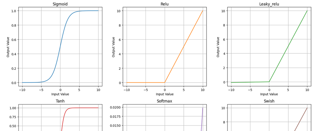
Bonus: Comparing all activation functions.

Here is the final version of python code if you want to compare all output

import numpy as np
import matplotlib.pyplot as plt

# Define the activation functions
def sigmoid(x):
    return 1 / (1 + np.exp(-x))

def relu(x):
    return np.maximum(0, x)

def leaky_relu(x, alpha=0.01):
    return np.maximum(alpha*x, x)

def tanh(x):
    return np.tanh(x)

def softmax(x):
    e_x = np.exp(x - np.max(x))  # subtract max(x) for numerical stability
    return e_x / e_x.sum(axis=0)

def swish(x):
    return x / (1 + np.exp(-x))

# Generate a range of values from -10 to 10
x = np.linspace(-10, 10, 1000)

# Create a list of all the activation functions
activations = [sigmoid, relu, leaky_relu, tanh, softmax, swish]

# Get a colormap
cmap = plt.get_cmap("tab10")

# Set the size of the full figure
plt.figure(figsize=(14, 8.8))

# Iterate over each activation function
for i, activation in enumerate(activations):
    # Create a subplot for this activation function
    plt.subplot(2, 3, i+1)
    # Apply the activation function and plot the result
    plt.plot(x, activation(x), color=cmap(i))
    plt.title(activation.__name__.capitalize())
    plt.xlabel("Input Value")
    plt.ylabel("Output Value")
    plt.grid(True)

# Adjust the layout and show the plot
plt.tight_layout()
plt.show()

Output

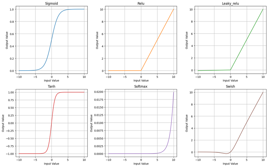
Note: The softmax function is a bit different because it normalizes the outputs to sum to 1, so the shape of its plot will differ from the others. It's generally used for multi-class classification tasks to provide a probability distribution over classes.