Understanding Feedforward Neural Network

Disclosure: Please note that the content in this blog was written with the assistance of OpenAI's ChatGPT language model.

A Feedforward Neural Network, also simply known as a Neural Network, is a type of artificial neural network where connections between the nodes do not form a cycle. This is different from recurrent neural networks.

When we say that "connections between the nodes do not form a cycle," we are referring to the structure of the network.

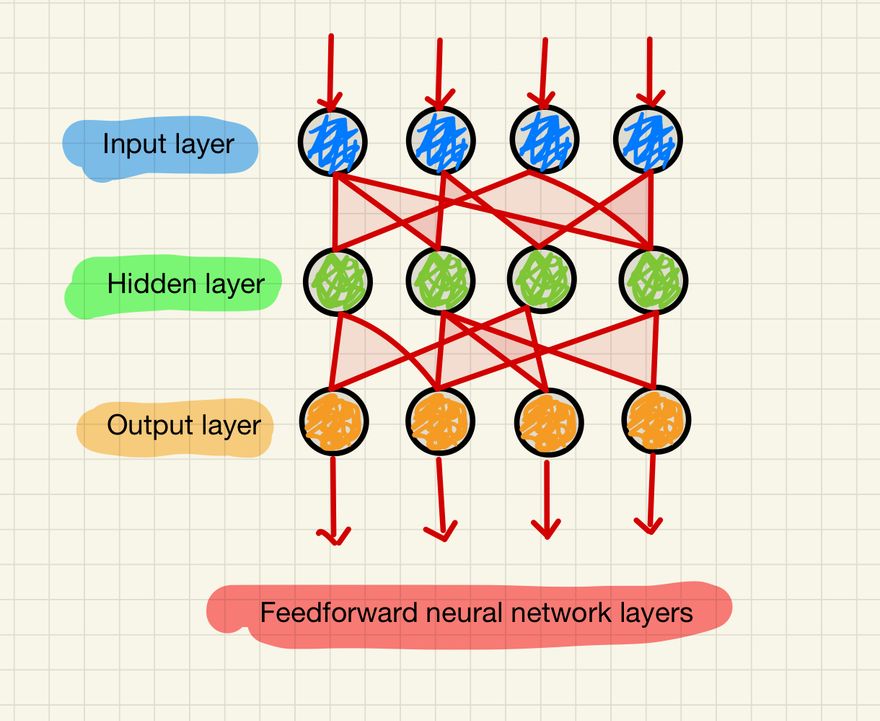
In a feedforward neural network, the information moves only in one direction: from the input layer, through the hidden layers, and finally to the output layer. There is no loop back from a higher layer to a lower layer. This unidirectional flow of data is what we mean by "no cycle."

For instance, consider three nodes A, B, and C. In a feedforward network, you might have connections from A to B and from B to C, but you would not have a connection from C back to A or B because that would create a cycle (A -> B -> C -> A).

In contrast, in a recurrent neural network (RNN), connections between nodes can form cycles. This means that information can flow in loops in the network, which is what allows RNNs to have a kind of "memory" of previous inputs. In the same scenario as above, in a recurrent network, it would be possible to have a connection from C back to A or B.

To visualize this, think of a feedforward neural network as a one-way street, where data can only move forward, while a recurrent neural network is like a roundabout, where data can circulate.

Here is a breakdown of its main components:

1. Nodes (or Neurons): The fundamental units of a neural network are nodes or neurons. These nodes take in input, apply a function to it, and then pass on the output.

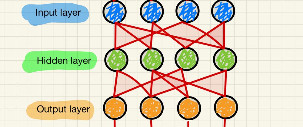
2. Layers:

   • Input Layer: This is where the network starts. Each node in this layer corresponds to one feature in your dataset.
   • Hidden Layer(s): These are located between the input and output layers. A network can have any number of hidden layers. These layers perform computations on the inputs received and transfer the result to the output layer.
   • Output Layer: This is where the final computations are done and the result/output is delivered.

3. Weights and Bias: Every input that enters a node has an associated weight which can be adjusted during learning, thereby affecting the importance or impact of an input. The bias allows you to shift the activation function curve up or down.

4. Activation Function: This is a function used to get the output of a node. It's used to introduce non-linearity into the output of a neuron. Examples include the sigmoid, tanh, and ReLU (Rectified Linear Unit) functions.

In a Feedforward Neural Network, the information only travels forward in the network. The data goes through the input nodes and passes through the hidden layers and finally through the output nodes. There are no loops in the network, i.e., the output of any layer does not affect that same layer.

A simple single-layer feedforward neural network would work as follows:

1. Each input node receives an input and multiplies it by a weight.
2. It adds a bias.
3. It then applies an activation function.
4. The resulting values are then sent forward to the next layer (or as the final output for a single-layer network).

The goal of training a feedforward neural network is to adjust the weights and biases to best map the input data to the correct output. This is usually done through a process called back propagation and an optimization strategy like gradient descent.

The key purposes of a neural network

• Approximate a Function: A key aspect of neural networks is their ability to approximate complex functions. This is essentially the foundation of machine learning – we're trying to find a function that can map our inputs (features) to our outputs (labels) with high accuracy. The optimal function is usually unknown and complex, so neural networks are used to approximate this function.

• Mapping that Finds Optimal Parameters: The mapping mentioned here refers to the process of adjusting the weights and biases in the network during training. These are the parameters of the function the network is approximating. Through a process like gradient descent and back propagation, the network iteratively adjusts these parameters to reduce the difference between its predicted output and the actual output.

• Layers of a Neural Network are a Directed Acyclic Graph (DAG): This refers to the structure of a feedforward neural network. A Directed Acyclic Graph is a structure that consists of nodes and edges, where each edge has a direction, and there are no cycles (a path that starts and ends at the same vertex). For a feedforward neural network, the nodes would be the neurons and the edges would be the connections between neurons. Information in this type of network always moves in one direction: from the input layer, through the hidden layers, and to the output layer, without looping back. This structure is why it's called a "feedforward" network.

How it works?

In a neural network, each node performs a calculation based on its input, weights, and bias, and then applies an activation function to that result. Let's denote:

• x as the input to the neuron
• w as the weights
• b as the bias
• a as the activation function

The output y of the neuron is calculated as follows:

y = a(w * x + b)

This is a vectorized form where x and w are vectors and the operation * is the dot product.

Single Layer Feedforward network example

Now, here is a very basic implementation of a single-layer feedforward neural network in Python:

import numpy as np

# Sigmoid activation function
def sigmoid(x):
    return 1 / (1 + np.exp(-x))

# Input array
X = np.array([[0, 0, 1],
              [0, 1, 1],
              [1, 0, 1],
              [1, 1, 1]])

# Output array
y = np.array([[0], [1], [1], [0]])

# Seed for random number generation
np.random.seed(1)

# Initialize weights with random values
weights = 2 * np.random.random((3, 1)) - 1

for iter in range(10000):
    # Forward propagation
    output = sigmoid(np.dot(X, weights))

    # Compute the error
    error = y - output

    # Back propagation (using the derivative of the sigmoid function)
    adjustment = error * (output * (1 - output))

    # Adjust the weights
    weights += np.dot(X.T, adjustment)

print("Output After Training:")
print(output)

Output:

Output After Training:
[[0.5]
 [0.5]
 [0.5]
 [0.5]]

In this example, we've created a basic neural network with one input layer and one output layer (thus, no hidden layers). The input layer has 3 neurons (as seen in the shape of X), and the output layer has 1 neuron (as seen in the shape of y). The weights are initialized randomly, and then the network is trained using a simple form of gradient descent, adjusting the weights based on the error between the predicted output and the actual output. The sigmoid function is used as the activation function for the neurons.

In this case our output is not making sense. The weights were randomly initialized and we've set the number of training iterations to 10,000. However, with this basic example and the configuration of the inputs and outputs (i.e., the XOR problem), it's likely the network wasn't able to correctly learn the function within these constraints.

A single layer neural network is unable to solve the XOR problem, which is a non-linearly separable problem, because it's essentially trying to draw a straight line to separate the inputs, which isn't possible. You'd need a multi-layer neural network (i.e., a neural network with at least one hidden layer) to solve the XOR problem.

Activation function sigmoid explained

The sigmoid function is a commonly used activation function in neural networks, especially for binary classification problems. It's defined as follows:

sigmoid(x) = 1 / (1 + exp(-x))

The sigmoid function takes a real-valued number and "squashes" it into range between 0 and 1. When the input is negative, the output is close to 0; when the input is positive, the output is close to 1. When the input is 0, the output is exactly 0.5.

This makes it a good choice for problems where you want the output to represent a probability, since probabilities must be between 0 and 1. This is why it's commonly used in the output layer of binary classification problems, where the goal is to predict the probability of the positive class.

Another key property of the sigmoid function is that it's differentiable everywhere, which is important for training neural networks using back-propagation. The derivative of the sigmoid function can be expressed in terms of the sigmoid function itself:

sigmoid_derivative(x) = sigmoid(x) * (1 - sigmoid(x))

This derivative function is used in the code example below during the back-propagation step, to adjust the weights based on the error of the network's output.

However, the sigmoid function has fallen out of favor for use in hidden layers, mainly due to two issues:
(1) vanishing gradients, where the gradients can become very small if the input is far from 0, which can slow down training or cause it to get stuck, and
(2) the output of the sigmoid function is not zero-centered, which can lead to undesirable zig-zagging dynamics in the gradient updates for the weights. Alternatives like the ReLU (Rectified Linear Unit) function or its variants are often used in hidden layers instead.

Multi-Layered Feedforward Neural Network

Here's a slightly more complex example that includes a hidden layer:

import numpy as np

# Sigmoid function
def sigmoid(x):
    return 1 / (1 + np.exp(-x))

# Derivative of the sigmoid function
def sigmoid_derivative(x):
    return x * (1 - x)

# Input dataset
X = np.array([[0, 0, 1],
              [0, 1, 1],
              [1, 0, 1],
              [1, 1, 1]])

# Output dataset
y = np.array([[0, 1, 1, 0]]).T

# Seed the random number generator
np.random.seed(1)

# Initialize weights randomly with mean 0 for the first layer (3 input nodes, 4 nodes in hidden layer)
weights0 = 2 * np.random.random((3, 4)) - 1

# Initialize weights for the second layer (4 nodes in hidden layer, 1 output node)
weights1 = 2 * np.random.random((4, 1)) - 1

for iter in range(10000):
    # Forward propagation
    layer0 = X
    layer1 = sigmoid(np.dot(layer0, weights0))
    layer2 = sigmoid(np.dot(layer1, weights1))

    # Calculate error
    layer2_error = y - layer2

    # Back propagation using the error and the derivative of the sigmoid function
    layer2_delta = layer2_error * sigmoid_derivative(layer2)
    layer1_error = layer2_delta.dot(weights1.T)
    layer1_delta = layer1_error * sigmoid_derivative(layer1)

    # Adjust weights
    weights1 += layer1.T.dot(layer2_delta)
    weights0 += layer0.T.dot(layer1_delta)

print("Output After Training:")
print(layer2)

This is an implementation of a 2-layer neural network (1 hidden layer and 1 output layer). This should correctly learn the function for the XOR problem, giving you an output close to [0, 1, 1, 0]. The exact values might not be 0 or 1 due to the sigmoid activation function outputting values between 0 and 1. But values close to 0 can be interpreted as 0 and values close to 1 can be interpreted as 1.

So in this case we are seeing following output,

[[0.00702213]
 [0.99100952]
 [0.99215162]
 [0.01047911]]

We can see that the first and last values are very close to 0, and the second and third values are very close to 1. This is effectively the same as [0, 1, 1, 0] in the context of binary classification.

In practice, when you're using a sigmoid activation function for binary classification, you would usually round the output to the nearest integer to get a definite 0 or 1 prediction. In this case, rounding the values would give you the expected [0, 1, 1, 0].