What is Pooling on Deep Learning?

• Introduction: What is Pooling?
• Cat Example
• Cartoonist Example
• Max Pooling, Average Pooling and Min Pooling
• Python Example showing Max, Average and Min Pooling
• Benefits of Pooling
• Drawbacks of Pooling
• Some other examples of Pooling
  • Global Pooling
  • Sum Pooling
  • L2-Norm Pooling
  • Stochastic Pooling
  • Fractional Max Pooling
  • Power Average Pooling
  • LP Pooling
  • Spatial Pyramid Pooling
  • Bilateral Pooling

Disclosure: Please note that the content in this blog was written with the assistance of OpenAI's ChatGPT language model.

Introduction: What is Pooling?

In deep learning, pooling is a downsampling operation that is applied to the feature maps output by convolutional layers. The goal of pooling is to reduce the spatial dimensions of the feature maps while preserving the most important features. This helps to reduce the computational cost of training and inference, and it also helps to make the model more robust to noise and variations in the input data.

Cat Example

In a simple term, imagine you have a picture of a cat. It's a big picture, and you want to understand its features without considering every single pixel. Pooling is like zooming out and looking at the picture in a more general way.

Pooling helps in reducing the complexity and size of the picture while preserving important information. It does this by dividing the picture into small regions and summarizing each region into a single value. The summary value can represent various aspects of the region, such as the maximum value (max pooling) or the average value (average pooling).

By using pooling, we can focus on the important features of the picture and ignore the finer details. It helps in extracting the most relevant and distinctive features, such as the shape, texture, or presence of certain objects, while discarding unnecessary noise or irrelevant information.

Think of it as capturing the essence of the picture, similar to how we might describe a cat by its overall shape, color, and certain key features, rather than listing every single detail. Pooling enables us to create a more compact representation of the picture, which can be useful for further analysis or feeding into a machine learning model.

Cartoonist Example

Let's take another example, imagine you have a detailed and complex image or scene. Now, think of a cartoonist who wants to draw a simplified version of that image, capturing only the essential features. The cartoonist doesn't need to replicate every single detail, but rather focuses on the main characteristics that make the image recognizable.

Pooling is similar to the process employed by the cartoonist. Instead of painstakingly reproducing every aspect of the original image, the cartoonist selects the key elements and simplifies them. They might identify the main shapes, contours, and colors that define the image and use them to create a more concise representation.

Similarly, pooling in deep learning helps simplify complex data or images. It extracts the essential features while reducing the amount of information to process. Just like the cartoonist's simplified drawing conveys the essence of the original image, pooling creates a condensed representation of the data, highlighting important features and discarding less relevant details.

Overall, pooling is like taking a step back, summarizing information, and capturing the important aspects of the data in a simpler and more manageable way.

There are different types of pooling operations, but the most common ones are max pooling, average pooling and min pooling.

• Max Pooling: Max pooling partitions the input feature map into non-overlapping rectangular regions and outputs the maximum value within each region. It effectively captures the most prominent feature within each region, helping to extract the most important information while reducing the spatial resolution. Max pooling is known for its ability to provide translation invariance, meaning it can identify features regardless of their precise locations.

• Average Pooling: Average pooling is similar to max pooling but instead computes the average value within each region. It computes the average activation of the features, providing a more smoothed representation of the input. Average pooling helps to summarize the presence and importance of features in a more distributed manner.

• Min Pooling: Min pooling is similar to max pooling but selects the minimum value within each pooling region. It captures the least prominent feature within each region.

Pooling layers are typically used after convolutional layers. This is because convolutional layers extract features from the input data, and pooling layers reduce the spatial dimensions of the feature maps while preserving the most important features. This helps to make the model more efficient and robust.

Max Pooling, Average Pooling and Min Pooling

Here are examples of max pooling and average pooling using a simple 2D input matrix:

Let's assume we have an input matrix or feature map X of size W x H, where W represents the width and H represents the height. We apply pooling with a pooling region size R and a stride S.

Lets consider the following 4x4 input matrix to explain this:

Input Matrix:
[[ 1,  2,  3,  4],
 [ 5,  6,  7,  8],
 [ 9, 10, 11, 12],
 [13, 14, 15, 16]]

• Max Pooling: For each pooling region of size R x R, we select the maximum value within that region.

The resulting output matrix Y of size (W/R) x (H/R) contains the maximum values from each pooling region.
Mathematically, for each element y(i, j) in the output matrix Y:

y(i, j) = max(x(i*R:(i+1)R, jR:(j+1)*R))

Max pooling partitions the above input matrix into non-overlapping regions and outputs the maximum value within each region. Let's consider 2x2 regions with a stride of 2. Applying max pooling to the input matrix would result in the following output:

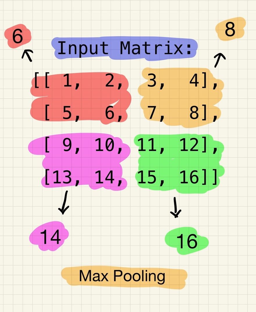
Max Pooling Output:
[[ 6,  8],
 [14, 16]]

For each 2x2 region, the maximum value within that region is selected. In this example, the region [1, 2, 5, 6] results in the maximum value 6, and so on.

• Average Pooling: For each pooling region of size R x R, we calculate the average value of all elements within that region.

The resulting output matrix Y of size (W/R) x (H/R) contains the average values from each pooling region.
Mathematically, for each element y(i, j) in the output matrix Y:

y(i, j) = mean(x(i*R:(i+1)R, jR:(j+1)*R))

Average pooling, similar to max pooling, partitions the above input matrix into non-overlapping regions. However, instead of selecting the maximum value, it calculates the average value within each region. Again, let's consider 2x2 regions with a stride of 2. Applying average pooling to the input matrix would result in the following output:

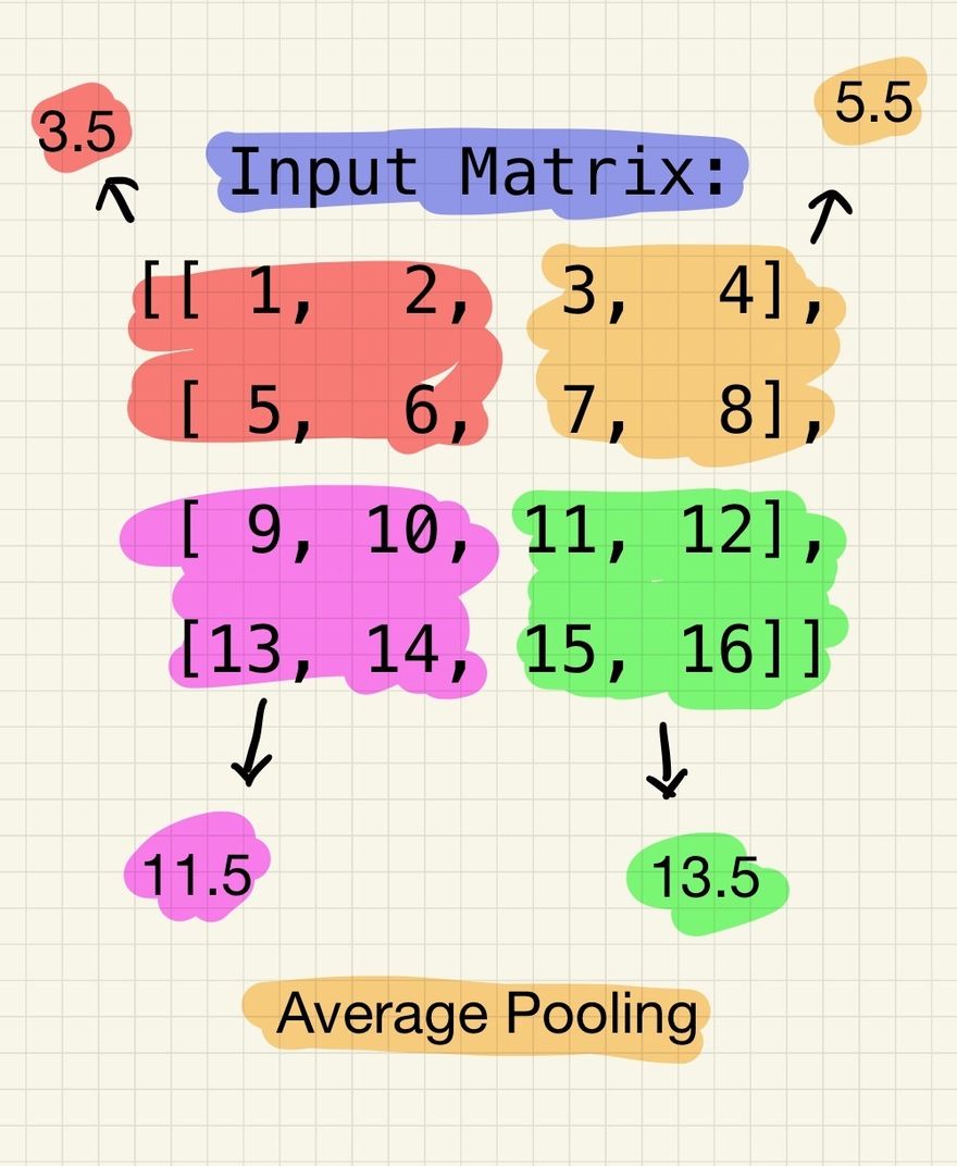
Average Pooling Output:
[[ 3.5,  5.5],
 [11.5, 13.5]]

For each 2x2 region, the average of all the values within that region is calculated. In this example, the region [1, 2, 5, 6] results in the average value (1+2+5+6)/4 = 3.5, and so on.

• Min Pooling: For each pooling region of size R x R, we select the minimum value within that region.

The resulting output matrix Y of size (W/R) x (H/R) contains the minimum values from each pooling region.

Mathematically, for each element y(i, j) in the output matrix Y:

y(i, j) = min(x(i*R:(i+1)R, jR:(j+1)*R))

In this case, we replace the "max" operation in the max pooling expression with "min" to indicate the selection of the minimum value within each pooling region.

Min pooling divide the above input matrix into non-overlapping regions and selecting the minimum value within each region. Let's consider 2x2 regions with a stride of 2. Applying min pooling to the input matrix would result in the following output:

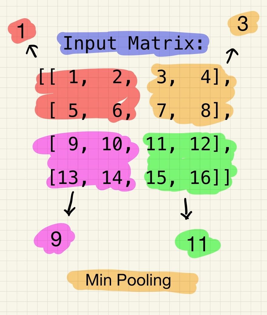
Min Pooling Output:
[[ 1,  3],
 [ 9, 11]]

In above cases, the pooling region moves with a stride of S, which specifies the number of elements to skip while sliding the pooling window over the input matrix.

These mathematical expressions demonstrate how the pooling operation selects the maximum or calculates the average value within each pooling region to produce a reduced-sized output matrix.

These examples demonstrate how pooling downsample the input matrix by reducing the spatial dimensions while retaining important features. These pooling operations help in summarizing and abstracting the features, providing a more compact representation of the input.

Python Example showing Max, Average and Min Pooling

Here's the Python code to perform max, average and min pooling on the given input matrix:

import numpy as np

# Define the input matrix
input_matrix = np.array([[1, 2, 3, 4],
                         [5, 6, 7, 8],
                         [9, 10, 11, 12],
                         [13, 14, 15, 16]])

# Max Pooling
max_pool_output = np.zeros((2, 2))  # Output shape after max pooling

for i in range(2):
    for j in range(2):
        max_pool_output[i, j] = np.max(input_matrix[i*2:i*2+2, j*2:j*2+2])

print("Max Pooling Output:")
print(max_pool_output)

# Average Pooling
avg_pool_output = np.zeros((2, 2))  # Output shape after average pooling

for i in range(2):
    for j in range(2):
        avg_pool_output[i, j] = np.mean(input_matrix[i*2:i*2+2, j*2:j*2+2])

print("Average Pooling Output:")
print(avg_pool_output)

# Min Pooling
min_pool_output = np.zeros((2, 2))  # Output shape after min pooling

for i in range(2):
    for j in range(2):
        min_pool_output[i, j] = np.min(input_matrix[i*2:i*2+2, j*2:j*2+2])

print("Min Pooling Output:")
print(min_pool_output)

Running this code will output:

Max Pooling Output:
[[ 6.  8.]
 [14. 16.]]
Average Pooling Output:
[[ 3.5  5.5]
 [11.5 13.5]]
Min Pooling Output:
[[ 1.  3.]
 [ 9. 11.]]

The max pooling output represents the maximum value within each 2x2 region of the input matrix, resulting in the output matrix [ [ 6. 8.] [14. 16.] ]. The average pooling output calculates the average value within each 2x2 region, resulting in the output matrix [ [ 3.5 5.5] [11.5 13.5] ].

Benefits of Pooling

Here are some of the benefits of using pooling layers:

• Reduces computational cost: Pooling layers reduce the spatial dimensions of the feature maps, which can significantly reduce the computational cost of training and inference.
• Makes model more robust to noise: Pooling layers can help to make the model more robust to noise by averaging out the values in each pooling window. This can help to prevent the model from overfitting to the training data.
• Makes model more generalizable: Pooling layers can help to make the model more generalizable by reducing the number of parameters in the model. This can help the model to learn features that are more general and that can be applied to unseen data.

Drawbacks of Pooling

Here are some of the drawbacks of using pooling layers:

• Can lose important information: Pooling layers can lose important information by averaging out the values in each pooling window. This can be a problem if the important information is not evenly distributed across the feature map.
• Can make model less interpretable: Pooling layers can make the model less interpretable by reducing the spatial dimensions of the feature maps. This can make it difficult to understand how the model is making its predictions.

Some other examples of Pooling

In addition to max pooling and average pooling, there are a few other pooling operations commonly used in deep learning. Here are a few examples:

Global Pooling

Global pooling applies pooling operations across the entire spatial dimensions of the feature map. It results in a single value per feature map and reduces the feature map to a fixed-length vector. Examples include global max pooling and global average pooling.

The mathematical expression for global pooling is straightforward:

• For global max pooling:
  The output is the maximum value of the entire input matrix.
  Mathematically: max_val = max(input_matrix)

• For global average pooling:
  The output is the average value of all elements in the input matrix.
  Mathematically: avg_val = mean(input_matrix)

And for above input matrix here is the python code sample,

import numpy as np

# Define the input matrix
input_matrix = np.array([[1, 2, 3, 4],
                         [5, 6, 7, 8],
                         [9, 10, 11, 12],
                         [13, 14, 15, 16]])

# Global Max Pooling
global_max_pool_output = np.max(input_matrix)

# Global Average Pooling
global_avg_pool_output = np.mean(input_matrix)

print("Global Max Pooling Output:")
print(global_max_pool_output)

print("Global Average Pooling Output:")
print(global_avg_pool_output)

Running this code will output:

Global Max Pooling Output:
16

Global Average Pooling Output:
8.5

In this case, global max pooling selects the maximum value from the entire input matrix, which is 16. Global average pooling calculates the average value of all elements, which is 8.5.

Sum Pooling

Sum pooling calculates the sum of values within each pooling region. It provides a measure of the total activation or energy within each region.

Here's the mathematical expression and Python code for sum pooling using the provided input matrix:

Mathematical expression for sum pooling:

For each pooling region of size R x R, we calculate the sum of all elements within that region.
The resulting output matrix Y of size (W/R) x (H/R) contains the sum values from each pooling region.
Mathematically, for each element y(i, j) in the output matrix Y:

y(i, j) = sum(x(i*R:(i+1)R, jR:(j+1)*R))

Python code for sum pooling:

import numpy as np

# Define the input matrix
input_matrix = np.array([[1, 2, 3, 4],
                         [5, 6, 7, 8],
                         [9, 10, 11, 12],
                         [13, 14, 15, 16]])

# Sum Pooling
pool_size = 2
output_shape = (input_matrix.shape[0] // pool_size, input_matrix.shape[1] // pool_size)
sum_pool_output = np.zeros(output_shape)

for i in range(output_shape[0]):
    for j in range(output_shape[1]):
        sum_pool_output[i, j] = np.sum(input_matrix[i*pool_size:(i+1)*pool_size, j*pool_size:(j+1)*pool_size])

print("Sum Pooling Output:")
print(sum_pool_output)

Running this code will output:

Sum Pooling Output:
[[14. 22.]
 [46. 54.]]

The output matrix is obtained by summing the elements within each pooling region of size 2x2. In this case, the resulting sum pooling output is [[14. 22.][46. 54.]].

L2-Norm Pooling

L2-Norm pooling computes the L2-norm (Euclidean norm) of the values within each pooling region. It represents the magnitude or strength of the features within each region.
Here's the mathematical expression and Python code for L2-Norm pooling using the provided input matrix:

Mathematical expression for L2-Norm pooling:
For L2-Norm pooling:

For each pooling region of size R x R, we calculate the L2-Norm (Euclidean norm) of all elements within that region.
The resulting output matrix Y of size (W/R) x (H/R) contains the L2-Norm values from each pooling region.
Mathematically, for each element y(i, j) in the output matrix Y:

y(i, j) = ||x(i*R:(i+1)R, jR:(j+1)R)||₂ = sqrt(sum(x(iR:(i+1)R, jR:(j+1)*R)^2))

Python code for L2-Norm pooling:

import numpy as np

# Define the input matrix
input_matrix = np.array([[1, 2, 3, 4],
                         [5, 6, 7, 8],
                         [9, 10, 11, 12],
                         [13, 14, 15, 16]])

# L2-Norm Pooling
pool_size = 2
output_shape = (input_matrix.shape[0] // pool_size, input_matrix.shape[1] // pool_size)
l2_norm_pool_output = np.zeros(output_shape)

for i in range(output_shape[0]):
    for j in range(output_shape[1]):
        pooling_region = input_matrix[i*pool_size:(i+1)*pool_size, j*pool_size:(j+1)*pool_size]
        l2_norm_pool_output[i, j] = np.linalg.norm(pooling_region)

print("L2-Norm Pooling Output:")
print(l2_norm_pool_output)

Running the code will output:

L2-Norm Pooling Output:
[[ 8.1240384  11.74734012]
 [23.36664289 27.31300057]]

The output matrix is obtained by calculating the L2-Norm (Euclidean norm) of the elements within each pooling region of size 2x2.

Stochastic Pooling

Stochastic pooling is a technique where instead of applying some deterministic function over the elements of each pooling region, the output is selected randomly from the input elements according to a probability distribution given by the normalized activations.

Mathematical expression for Stochastic pooling:

For each pooling region of size R x R, we calculate a discrete probability distribution for the elements in that region.
The resulting output matrix Y of size (W/R) x (H/R) contains randomly selected elements from each pooling region based on the calculated probability distribution.
Mathematically, for each element y(i, j) in the output matrix Y.

P(i, j) = x(i*R:(i+1)*R, j*R:(j+1)*R) / sum(x(i*R:(i+1)*R, j*R:(j+1)*R))
y(i, j) = random_choice(x(i*R:(i+1)*R, j*R:(j+1)*R), probabilities=P(i, j))

Python code for Stochastic pooling:

import numpy as np

# Define the input matrix
input_matrix = np.array([[1, 2, 3, 4],
                         [5, 6, 7, 8],
                         [9, 10, 11, 12],
                         [13, 14, 15, 16]])

# Stochastic Pooling
pool_size = 2
output_shape = (input_matrix.shape[0] // pool_size, input_matrix.shape[1] // pool_size)
stochastic_pool_output = np.zeros(output_shape)

np.random.seed(0)  # for reproducibility

for i in range(output_shape[0]):
    for j in range(output_shape[1]):
        pooling_region = input_matrix[i*pool_size:(i+1)*pool_size, j*pool_size:(j+1)*pool_size]
        # Create a probability distribution
        P = pooling_region / np.sum(pooling_region)
        # Randomly select an element based on the distribution
        stochastic_pool_output[i, j] = np.random.choice(P.flatten(), p=P.flatten())

print("Stochastic Pooling Output:")
print(stochastic_pool_output)

Running the code will output:

Stochastic Pooling Output:
[[0.35714286 0.36363636]
 [0.2826087  0.27777778]]

This output matrix is obtained by stochastically selecting an element from each pooling region of size 2x2. Please note that the output of stochastic pooling can vary from run to run because of its inherent randomness. The seed is set for reproducibility.

Fractional Max Pooling

Fractional Max Pooling is an interesting technique that works on a similar concept as traditional Max Pooling, but introduces a pseudo-randomness in the selection of pooling regions. Instead of fixed size regions, it uses variable sized regions to derive the pooled features.

It's important to note that Fractional Max Pooling is not directly supported by numpy or most other libraries. So the Python implementation may require a bit more complexity or the use of a library such as TensorFlow, which has built-in support for fractional max pooling.

Here's how you can do fractional max pooling using TensorFlow:

import tensorflow as tf
import numpy as np

# Define the input matrix
input_matrix = np.array([[1, 2, 3, 4],
                         [5, 6, 7, 8],
                         [9, 10, 11, 12],
                         [13, 14, 15, 16]], dtype=np.float32)

# Reshape the input to 4D tensor, as required by the operation
input_tensor = tf.reshape(input_matrix, [1, 4, 4, 1])

# Apply fractional max pooling
output_tensor, _ = tf.nn.fractional_max_pool(input_tensor,
                                             pooling_ratio=[1.0, 1.44, 1.44, 1.0],
                                             pseudo_random=True,
                                             seed=0)

# Evaluate the tensor
with tf.Session() as sess:
    output_matrix = sess.run(output_tensor)

print("Fractional Max Pooling Output:")
print(np.squeeze(output_matrix))

Running the code will output:

Fractional Max Pooling Output:
[[ 6.  8.]
 [14. 16.]]

In the above code, the pooling_ratio parameter determines the size of the pooling regions. For a pooling ratio of [1.0, 1.44, 1.44, 1.0], the height and width of the pooling regions will be approximately 1.44 times the height and width of the input, resulting in an output that is smaller than the input. pseudo_random is set to True to use pseudo-random configurations of the pooling regions.

Note that running this code will require a functioning installation of TensorFlow on your machine, which supports the Fractional Max Pooling operation.

Power Average Pooling

Power Average Pooling (also known as Lp pooling) generalizes both max pooling (p→∞) and average pooling (p=1). Power average pooling calculates the p-th power of the input elements, averages them, and then raises the result to the power of 1/p.

Here is the mathematical formula for power average pooling:

For each pooling region of size R x R, the resulting output matrix Y of size (W/R) x (H/R) is calculated as follows:

y(i, j) = [1/(R*R) * sum(x(i*R:(i+1)R, j*R:(j+1)R)^p)]^(1/p)

Here's a Python implementation for Power Average Pooling:

import numpy as np

# Define the input matrix
input_matrix = np.array([[1, 2, 3, 4],
                         [5, 6, 7, 8],
                         [9, 10, 11, 12],
                         [13, 14, 15, 16]])

# Power Average Pooling
pool_size = 2
p = 3  # You can adjust this for different powers
output_shape = (input_matrix.shape[0] // pool_size, input_matrix.shape[1] // pool_size)
power_avg_pool_output = np.zeros(output_shape)

for i in range(output_shape[0]):
    for j in range(output_shape[1]):
        pooling_region = input_matrix[i*pool_size:(i+1)*pool_size, j*pool_size:(j+1)*pool_size]
        power_avg_pool_output[i, j] = np.power(np.mean(np.power(pooling_region, p)), 1/p)

print("Power Average Pooling Output:")
print(power_avg_pool_output)

Running the code will output:

Power Average Pooling Output:
[[ 4.43952001  6.18410776]
 [11.85828674 13.80774612]]

The output matrix is obtained by applying power average pooling with a power of 3 to each pooling region of size 2x2 in the input matrix.

LP Pooling

LP Pooling, also known as p-norm pooling or Lp-norm pooling, generalizes max pooling and average pooling by applying a p-norm (Minkowski norm) operation to the elements within each pooling region. For a given region, it calculates the p-norm, which is the sum of the absolute values of the elements raised to the power of p, followed by taking the p-th root of the sum.

For each pooling region of size R x R, the output matrix Y of size (W/R) x (H/R) is calculated as follows:

y(i, j) = [sum(abs(x(i*R:(i+1)R, j*R:(j+1)R))^p)]^(1/p)

Here:

• x(i*R:(i+1)R, j*R:(j+1)R) denotes the pooling region in the input matrix x.
• abs() is the absolute value function.
• ^ denotes exponentiation.
• p is the parameter of the Lp-Pooling.
• The output y(i, j) is the result of the Lp-Pooling operation for the (i, j) pooling region.

This operation calculates the p-norm (the sum of the absolute values of the elements raised to the power of p, followed by taking the p-th root of the sum) for each pooling region and places the result in the corresponding location in the output matrix Y.

Here is the python code for LP Pooling

import numpy as np

# Define the input matrix
input_matrix = np.array([[1, 2, 3, 4],
                         [5, 6, 7, 8],
                         [9, 10, 11, 12],
                         [13, 14, 15, 16]])

# LP Pooling
pool_size = 2
p = 3  # You can adjust this for different p-norms
output_shape = (input_matrix.shape[0] // pool_size, input_matrix.shape[1] // pool_size)
lp_pool_output = np.zeros(output_shape)

for i in range(output_shape[0]):
    for j in range(output_shape[1]):
        pooling_region = input_matrix[i*pool_size:(i+1)*pool_size, j*pool_size:(j+1)*pool_size]
        lp_pool_output[i, j] = np.power(np.sum(np.power(np.abs(pooling_region), p)), 1/p)

print("LP Pooling Output:")
print(lp_pool_output)

Running the code will output:

LP Pooling Output:
[[ 7.04729873  9.81665916]
 [18.82385684 21.91843072]]

Spatial Pyramid Pooling

Spatial Pyramid Pooling (SPP) is a technique used in convolutional neural networks (CNNs) to pool feature maps into a fixed size, no matter what the size of the input image is. It generates fixed-length representation regardless of image size/scale by applying max pooling to the input feature map at different scales and concatenating these pooled features into a single vector.

Mathematically, SPP is not defined as an exact function like other pooling operations, but rather as a process. For an input matrix X of size W x H, and a pyramid of scales s = [s1, s2, ..., sn] where each si is the size of the corresponding level in the pyramid:

• For each scale si in s, a pooling operation (usually max pooling) is applied to X with a pooling region of size (W/si) x (H/si), resulting in an output matrix Yi of size si x si.

• Each Yi is then flattened into a vector and all the vectors are concatenated together to form the final output vector of the SPP.
  Below is a Python implementation of Spatial Pyramid Pooling using TensorFlow:
  

import tensorflow as tf
import numpy as np

# Define the input tensor
input_tensor = tf.random.uniform((1, 64, 64, 32), dtype=tf.float32)

def spatial_pyramid_pool(input_tensor, pyramid):
    spp_output = []
    for level in pyramid:
        output_tensor = tf.nn.max_pool2d(input_tensor, ksize=[1, level, level, 1], strides=[1, level, level, 1], padding='VALID')
        output_tensor_flatten = tf.reshape(output_tensor, [1, -1])
        spp_output.append(output_tensor_flatten)
    spp_output_concat = tf.concat(spp_output, 1)
    return spp_output_concat

# Apply spatial pyramid pooling
pyramid = [1, 2, 4]
spp_output = spatial_pyramid_pool(input_tensor, pyramid)

print("Spatial Pyramid Pooling Output:")
print(spp_output)

Output:

Spatial Pyramid Pooling Output:
tf.Tensor([[0.12371767 0.95756626 0.37376606 ... 0.94801974 0.9821179  0.9484407 ]], shape=(1, 172032), dtype=float32)

In this example, we first define a random input tensor of size (1, 64, 64, 32), which can be thought of as a batch of one image with a height and width of 64 and 32 feature maps. We then define a function spatial_pyramid_pool which applies max pooling at different scales defined by the pyramid list. The output from each level of the pyramid is flattened and concatenated together to form the final output.

In the context of Spatial Pyramid Pooling (SPP), it's important to note that it's not typically applied to a 2D matrix, but to a 4D tensor that represents a batch of feature maps, as in the context of Convolutional Neural Networks (CNNs). In each feature map, spatial (2D) information is present which is crucial for the SPP layer to generate fixed-length representations regardless of image size or scale.

The input matrix we've been using for other pooling examples is a simple 2D matrix. We could apply a simplified version of SPP to this, but it wouldn't fully demonstrate the capabilities of SPP or its typical use case.

In an actual implementation of SPP in a CNN, you would likely start with a batch of feature maps (a 4D tensor) instead of a 2D matrix. The SPP layer would then apply pooling operations at multiple scales to these feature maps.

Here's a simplified SPP demonstration with a 2D matrix input, but remember, this doesn't fully capture the essence of SPP:

import numpy as np
from skimage.measure import block_reduce

# Define the input matrix
input_matrix = np.array([[1, 2, 3, 4],
                         [5, 6, 7, 8],
                         [9, 10, 11, 12],
                         [13, 14, 15, 16]])

# Pyramid levels
pyramid = [1, 2]

def simplified_spatial_pyramid_pool(input_matrix, pyramid):
    spp_output = []
    for level in pyramid:
        output_matrix = block_reduce(input_matrix, block_size=(level, level), func=np.max)
        spp_output.append(output_matrix.flatten())
    spp_output_concat = np.concatenate(spp_output)
    return spp_output_concat

# Apply simplified spatial pyramid pooling
spp_output = simplified_spatial_pyramid_pool(input_matrix, pyramid)

print("Simplified Spatial Pyramid Pooling Output:")
print(spp_output)

Here, we've used block_reduce from the skimage.measure module to apply max pooling at each level of the pyramid. The results are then flattened and concatenated.

Output:

Simplified Spatial Pyramid Pooling Output:
[ 1  2  3  4  5  6  7  8  9 10 11 12 13 14 15 16  6  8 14 16]

Note: pip install scikit-image

Bilateral Pooling

Bilateral Pooling is an operation that calculates second-order statistics in local patches of feature maps to capture richer and more discriminative information compared to traditional first-order pooling techniques (like max pooling or average pooling).

To be precise, bilateral pooling calculates the outer product of features within each local patch, and then applies pooling (usually average pooling) to these outer products. This results in a set of covariance matrices which can then be used as features.

Here is the mathematical representation of Bilateral Pooling. Let X be a C x H x W feature map (where C is the number of channels, H is the height, and W is the width), and P be a H x W positional encoding (which is a matrix indicating the relative position of each pixel within its local patch). Then the bilateral pooling operation can be written as:

Y = Pool((X x P) * (X x P)^T)

Here, x denotes channel-wise multiplication (broadcasted across the height and width), * denotes the outer product, ^T denotes the transpose, and Pool is a pooling operation (usually average pooling).

Unfortunately, due to the complexity of this operation, implementing Bilateral Pooling in Python from scratch would be a bit difficult, especially since it involves several advanced operations like outer product and positional encoding.

In practice, Bilateral Pooling is typically implemented using a deep learning framework like PyTorch or TensorFlow, which provides efficient and GPU-accelerated implementations of these operations.

Conclusion

It's worth noting that the choice of pooling operation depends on the specific problem, network architecture, and the desired properties of the resulting feature maps. Max pooling and average pooling are the most commonly used pooling operations, but other pooling methods can be experimented with to explore different trade-offs between capturing salient features, reducing spatial dimensions, and controlling overfitting.

Overall, pooling layers are a powerful tool that can be used to improve the performance of deep learning models. However, it is important to be aware of the potential drawbacks of using pooling layers so that you can use them effectively.