What is Regularization on Machine Learning? Lasso vs Ridge Regression

Disclosure: Please note that the content in this blog was written with the assistance of OpenAI's ChatGPT language model.

What is Regularization, Text Book definition

Regularization is a technique used in machine learning to prevent overfitting, which occurs when the model learns the training data too well and performs poorly on unseen data, like the test or validation set. Overfitting typically happens when the model is excessively complex, such as having too many parameters.

Regularization works by adding a penalty term to the loss function, which the model aims to minimize during training. This penalty term discourages the model from assigning too much importance to any one feature, thereby reducing the complexity of the model.

There are different types of regularization, including L1 regularization, L2 regularization, and dropout.

• L1 regularization (Lasso regression): The penalty term is the absolute value of the magnitude of coefficients. This can result in some coefficients being reduced to zero, effectively removing the corresponding feature from the model.

• L2 regularization (Ridge regression): The penalty term is the square of the magnitude of coefficients. This generally results in smaller coefficients, but it doesn't eliminate them completely.

• Dropout: This is a different type of regularization used primarily in neural networks. During training, some percentage of nodes in a layer are randomly "dropped out," or temporarily deactivated. This prevents the model from relying too heavily on any one node and encourages it to learn more robust features.

Regularization is a key concept in machine learning and can significantly improve model generalization, or the ability of the model to perform well on unseen data.

Let's consider some analogies to understand regularization in simple terms:

• Playing a Sport (Teamwork as Regularization): Imagine a basketball team where one player is significantly better than the others. The team becomes over-reliant on this player, passing the ball to him most of the time. However, if this player gets injured or has a bad day, the team's performance suffers a lot because they're not used to playing without him. Regularization in this context would be like a coach encouraging the team to distribute the ball more evenly and involve all players, so that the team's performance doesn't depend too heavily on any single player.

• Cooking (Spice Balance as Regularization): Imagine you are making a soup and there are many different spices you can add. If you add too much of one spice, the soup might be overwhelmed by that particular flavor. Regularization is like trying to create a well-balanced soup by preventing any one spice from dominating the flavor, ensuring that no single ingredient (or feature) dominates the outcome.

In both these examples, the idea is to avoid relying too heavily on one thing (a player in basketball or a spice in cooking) for the best outcome.

In terms of machine learning models:

• Without Regularization: You train a model to predict house prices based on features like square footage, number of bedrooms, location, etc. The model ends up placing a huge importance on square footage and ignores other features. As a result, it predicts prices inaccurately for houses that are smaller but in prime locations or have luxurious amenities.

• With Regularization: You add a regularization term to your model. Now, during training, the model tries to balance the weight given to all features rather than relying too heavily on square footage. The model might now pay more attention to features like location and number of bedrooms as well. As a result, it predicts more accurate prices for a wider range of houses.

What is Overfitting and why we should prevent it?

In above definition we introduce a term called Overfitting.
Overfitting in machine learning occurs when a model learns the training data too well. It essentially memorizes the data, including the noise and outliers, to such an extent that it performs poorly on new, unseen data.

Here's a simple analogy: Suppose you're studying for a history exam by doing practice questions. Overfitting would be like memorizing the answers to the practice questions without understanding the underlying concepts. You might do well if the exact same questions appear on the exam, but if the exam has different questions (even on the same topics), you'll probably do poorly.

Now, why is it important to prevent overfitting?

We usually build machine learning models to make predictions on new, unseen data. If a model is overfitting to the training data, it's not learning the underlying patterns in the data; it's just memorizing the training examples. This means it won't generalize well to new data, which is typically our ultimate goal.

We want our model to understand the overall pattern or trend in the data, rather than focusing on the specific details of the training data. Regularization is one of the techniques that help us achieve this balance, by adding a penalty for complexity in the model, and thus discouraging overfitting.

To illustrate, in the context of a student studying for an exam, the goal is not to memorize the textbooks but to understand the subject matter so that the student can apply their knowledge to new problems. Regularization is akin to encouraging the student to understand the concepts rather than memorize the details.

In machine learning, this balance is often referred to as the bias-variance tradeoff. A model with high bias oversimplifies the data and performs poorly because it doesn't learn enough from the training data (underfitting). A model with high variance overcomplicates the data and performs poorly because it learns too much from the training data (overfitting). The goal is to find a balance between bias and variance where the model performs well on both the training data and new, unseen data.

Let's demonstrate this by creating a simple example using polynomial regression, a type of linear regression where the relationship between the independent variable x and the dependent variable y is modeled as an nth degree polynomial.

Polynomial regression can easily result in overfitting if the degree of the polynomial is too high. Here's how we can illustrate this:

import numpy as np
import matplotlib.pyplot as plt
from sklearn.pipeline import make_pipeline
from sklearn.preprocessing import PolynomialFeatures
from sklearn.linear_model import LinearRegression

# Set a seed for reproducibility
np.random.seed(0)

# Generate some data
X = np.sort(np.random.rand(15))
y = np.sin(2 * np.pi * X) + np.random.randn(15) * 0.2

X_test = np.linspace(0, 1, 100)

# Underfitting model (degree 1)
model_1 = make_pipeline(PolynomialFeatures(1), LinearRegression())
model_1.fit(X[:, np.newaxis], y)

# Appropriate fitting model (degree 3)
model_3 = make_pipeline(PolynomialFeatures(3), LinearRegression())
model_3.fit(X[:, np.newaxis], y)

# Overfitting model (degree 10)
model_10 = make_pipeline(PolynomialFeatures(10), LinearRegression())
model_10.fit(X[:, np.newaxis], y)

# Plotting
fig, axs = plt.subplots(2, 2, figsize=(18, 10))

# Degree 1
axs[0, 0].scatter(X, y, color='black', label='data')
axs[0, 0].plot(X_test, model_1.predict(X_test[:, np.newaxis]), label='Underfitting (degree 1)', color='red')
axs[0, 0].legend(loc='best')
axs[0, 0].set_title('Underfitting (degree 1)')

# Degree 3
axs[0, 1].scatter(X, y, color='black', label='data')
axs[0, 1].plot(X_test, model_3.predict(X_test[:, np.newaxis]), label='Appropriate fit (degree 3)', color='green')
axs[0, 1].legend(loc='best')
axs[0, 1].set_title('Appropriate fit (degree 3)')

# Degree 10
axs[1, 0].scatter(X, y, color='black', label='data')
axs[1, 0].plot(X_test, model_10.predict(X_test[:, np.newaxis]), label='Overfitting (degree 10)', color='blue')
axs[1, 0].legend(loc='best')
axs[1, 0].set_title('Overfitting (degree 10)')

# Combined
axs[1, 1].scatter(X, y, color='black', label='data')
axs[1, 1].plot(X_test, model_1.predict(X_test[:, np.newaxis]), label='Underfitting (degree 1)', color='red')
axs[1, 1].plot(X_test, model_3.predict(X_test[:, np.newaxis]), label='Appropriate fit (degree 3)', color='green')
axs[1, 1].plot(X_test, model_10.predict(X_test[:, np.newaxis]), label='Overfitting (degree 10)', color='blue')
axs[1, 1].legend(loc='best')
axs[1, 1].set_title('Combined')

plt.tight_layout()
plt.show()

Output:

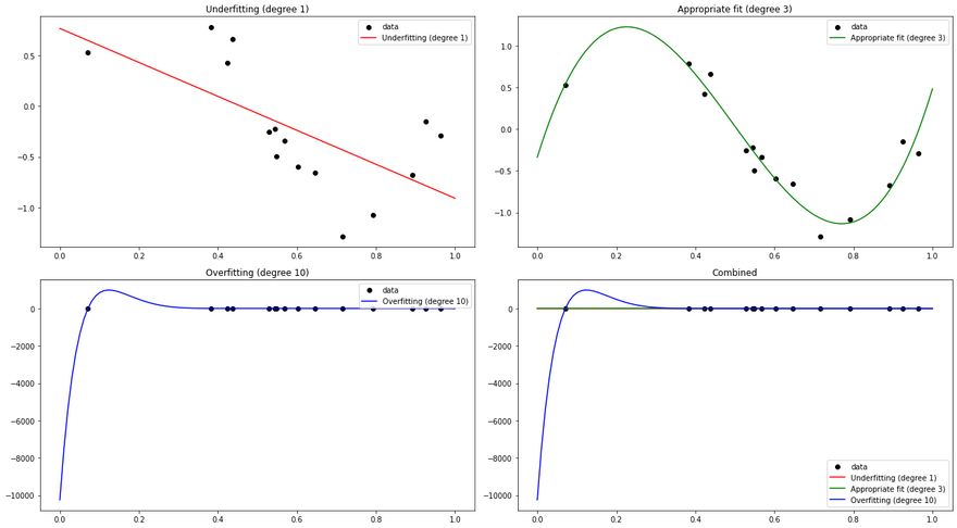
In this example, we first generate some random data following a sine curve. We then fit three different polynomial regression models to this data:

• A degree 1 model (essentially a simple linear regression), which is an underfitting model. It's too simple and cannot capture the underlying pattern of the data.
• A degree 3 model, which fits the data appropriately. It's complex enough to capture the pattern of the data, but not so complex that it overfits.
• A degree 10 model, which is an overfitting model. It's too complex and fits the noise in the data, leading to poor generalization on unseen data.

We plot the predictions of these three models along with the original data. You can see that the degree 1 model is too simple to capture the sine curve, the degree 3 model captures it well, and the degree 10 model is too flexible and fits the noise in the data, which is a classic sign of overfitting.

Let's linger little bit more into different types of regularization,

L1 Regularization (Lasso regression)

In L1 regularization, the penalty added to the loss function is the absolute value of the magnitude of the coefficients (weights).

For a simple linear regression with two parameters, the loss function with L1 regularization becomes:

L(θ) + λ|θ|

Here L(θ) is the original loss function, θ represents the coefficients (weights), and λ is the regularization parameter that controls the strength of the regularization penalty. The "|" denotes absolute value.

The L1 penalty has the effect of forcing some of the feature weights to be set to zero, effectively excluding them from the model. This leads to sparse solutions, which is useful in feature selection when dealing with high dimensional data.

Here's a simple Python code snippet using scikit-learn's Lasso function, which performs linear regression with L1 regularization:

import seaborn as sns
import matplotlib.pyplot as plt
import pandas as pd
from sklearn.linear_model import LogisticRegression
from sklearn.datasets import make_classification
from sklearn.model_selection import train_test_split
from sklearn.metrics import accuracy_score

# Generate a dataset with 100 samples and 20 features
X, y = make_classification(n_samples=100, n_features=20, n_informative=3)

# Split the dataset into a training set and a test set
X_train, X_test, y_train, y_test = train_test_split(X, y, test_size=0.2, random_state=42)

# Create a logistic regression model with L1 regularization
model = LogisticRegression(penalty='l1', solver='liblinear', C=0.1)
model.fit(X_train, y_train)

# Coefficients into DataFrame for plotting
coefficients = pd.DataFrame(model.coef_.reshape(-1, 1), columns=['Coefficient Value'])

# Visualize coefficients using seaborn lineplot
plt.figure(figsize=(10, 6))
sns.lineplot(x=coefficients.index, y=coefficients['Coefficient Value'])
plt.title('Feature Coefficients with L1 Regularization')
plt.show()

# Print the coefficients
print("Coefficients:", model.coef_)

# Coefficients into DataFrame for plotting
coefficients = pd.DataFrame(model.coef_.reshape(-1, 1), columns=['Coefficient Value'])

# Test the model
y_pred = model.predict(X_test)
print("Accuracy:", accuracy_score(y_test, y_pred))

# calculate the mean squared error of the predictions
mse = mean_squared_error(y_test, y_pred)
print(f'Mean Squared Error: {mse}')

Output:

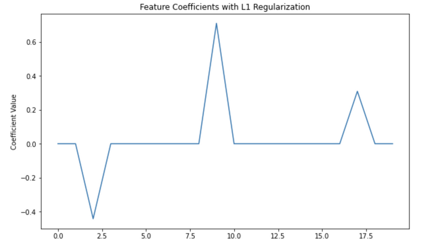
Coefficients: [[ 0.          0.         -0.44196177  0.          0.          0.
   0.          0.          0.          0.70979836  0.          0.
   0.          0.          0.          0.          0.          0.30909023
   0.          0.        ]]
Accuracy: 0.9
Mean Squared Error: 0.1

In this code, alpha is the λ in our equation (L(θ) + λ|θ|), which controls the strength of the regularization. You can increase alpha to increase the strength of the regularization, which will set more coefficients to zero.

A real-world example of where L1 regularization could be used is in genetic research. Suppose a scientist has a dataset where each sample is a person's genome, made up of 20,000 genes, and they want to find out which genes are most associated with a particular disease. They could train a model to predict disease status based on the person's genes and use L1 regularization to force the model to only select a small number of genes. The genes that the model uses would then be good candidates for further research.

L2 Regularization (Ridge regression)

In L2 regularization, the penalty added to the loss function is the square of the magnitude of the coefficients (weights).

For a simple linear regression with two parameters, the loss function with L2 regularization becomes:

L(θ) + λθ^2

Here, L(θ) is the original loss function, θ represents the coefficients (weights), and λ is the regularization parameter that controls the strength of the regularization penalty.

The effect of the L2 penalty is to constrain the values of the weights, effectively shrinking them towards zero, but not setting any of them exactly to zero. This means all features are included in the model, but the influence of less important features is reduced.

Here's a Python code snippet using scikit-learn's Ridge function, which performs linear regression with L2 regularization:

from sklearn.linear_model import Ridge
from sklearn.datasets import make_regression
from sklearn.model_selection import train_test_split
from sklearn.metrics import mean_squared_error

# Generate a dataset with 1000 samples and 10 features
X, y = make_regression(n_samples=1000, n_features=10, noise=0.1)

# Split the dataset into a training set and a test set
X_train, X_test, y_train, y_test = train_test_split(X, y, test_size=0.2, random_state=42)

# Apply Ridge regression (L2 regularization)
ridge = Ridge(alpha=0.1)
ridge.fit(X_train, y_train)

# Coefficients into DataFrame for plotting
coefficients = pd.DataFrame(ridge.coef_.reshape(-1, 1), columns=['Coefficient Value'])

# Visualize coefficients using seaborn
plt.figure(figsize=(10, 6))
sns.lineplot(x=coefficients.index, y=coefficients['Coefficient Value'])
plt.title('Feature Coefficients with L2 Regularization')
plt.show()


# Print the coefficients
print("Coefficients:", ridge.coef_)

# Make predictions on test data
y_pred = ridge.predict(X_test)

# Calculate the mean squared error of the predictions
mse = mean_squared_error(y_test, y_pred)
print('Mean Squared Error:', mse)

Output:

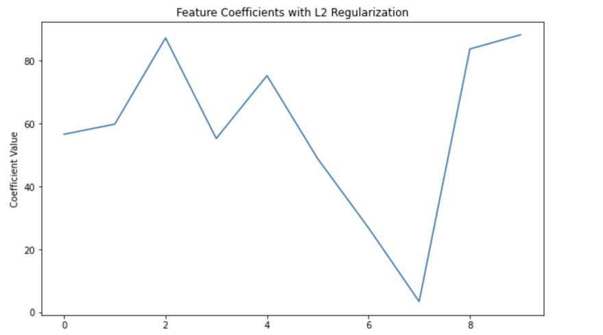
Coefficients: [56.55860496 59.76291192 87.16557359 55.21284729 75.18740404 48.79011741
 26.86870658  3.41227262 83.63555909 88.16793739]
Mean Squared Error: 0.009146818858695194

In this code, alpha is the λ in our equation (L(θ) + λθ^2), which controls the strength of the regularization.

A real-world example of where L2 regularization could be used is in a housing price prediction model. Suppose you have many features such as size of the house, number of bedrooms, number of bathrooms, distance from city center, age of the house, etc. Not all features are equally important, but all might have some effect on the house price. In this case, you might want to use L2 regularization to ensure that your model doesn't overly rely on any single feature, but still uses all of them to some degree.

Dropout

During the training phase, dropout randomly "drops out" (sets to zero) a number of output features of the layer during each training step. The "dropout rate" is the fraction of the features that are zeroed out; it's usually set between 0.2 and 0.5. At test time, no units are dropped out, but instead the layer's output values are scaled down by a factor equal to the dropout rate, to balance for the fact that more units are active than at training time.

The intuition behind dropout is that by randomly dropping out neurons, the neural network is forced to learn more robust features that are useful in conjunction with many different random subsets of the other neurons.

There isn't a straightforward mathematical expression for dropout as it's a stochastic (random) process, but if we denote the output of a layer as x and the output after applying dropout as y, we could express it as:

y_i = x_i * Bernoulli(p), for each i

where Bernoulli(p) is a Bernoulli random variable (which takes value 1 with probability p and 0 with probability 1-p), and p is the probability of keeping a neuron active.

Here's how you would implement dropout in a neural network using TensorFlow:

import tensorflow as tf
from sklearn.model_selection import train_test_split
from sklearn.datasets import make_classification

# generate some example classification data
X, y = make_classification(n_samples=1000, n_features=20, n_informative=15, n_redundant=5, random_state=7)

# split data into training and test set
X_train, X_test, y_train, y_test = train_test_split(X, y, test_size=0.2, random_state=42)

# build the model
model = tf.keras.models.Sequential([
  tf.keras.layers.Dense(64, activation='relu', input_shape=(20,)),  # input layer
  tf.keras.layers.Dropout(0.5),  # dropout layer
  tf.keras.layers.Dense(64, activation='relu'),  # hidden layer
  tf.keras.layers.Dropout(0.5),  # dropout layer
  tf.keras.layers.Dense(1, activation='sigmoid')  # output layer
])

# compile the model
model.compile(optimizer='adam', loss='binary_crossentropy', metrics=['accuracy'])

# train the model
model.fit(X_train, y_train, epochs=10, batch_size=32, validation_data=(X_test, y_test))

In this code, tf.keras.layers.Dropout(0.5) adds a dropout layer that sets half of the input units to 0 during training. This helps to prevent overfitting by ensuring that the model doesn't rely too heavily on any one feature.

A real-world example of dropout could be in image classification. Suppose you have a model trained to recognize dogs and it's overfitting, relying too heavily on specific pixels or regions of the image. By using dropout, you force the model to spread out its attention and consider multiple regions of the image, making it more robust and generalizable to unseen data.

Lasso Vs Ridge Regression

Here are some key differences between L1 and L2 regularization:

• Effect on Model Complexity: Both L1 and L2 regularization add a penalty to the loss function, which discourages large coefficients and therefore reduces model complexity. However, they do this in different ways.

• Sparsity: L1 regularization can produce sparse models, where some coefficients are exactly zero. This is because the absolute value penalty in L1 encourages coefficients to go to zero. In contrast, L2 regularization tends to distribute the coefficient values more evenly and results in small but non-zero coefficients. Thus, L1 regularization can be used for feature selection, while L2 regularization generally cannot.

• Solution Uniqueness: L2 regularization has a squared penalty which is strictly convex, so it always has a unique solution. L1 regularization, with its absolute value penalty, is not strictly convex and can have multiple solutions when several features are correlated.

• Robustness: L1 regularization is more robust to outliers than L2 regularization. This is because L2 regularization squares the errors, so it is more sensitive to outliers than L1 regularization.

• Computational Efficiency: L2 regularization has a closed-form solution, while L1 regularization does not. This can make models with L2 regularization faster to train. However, L1 regularization can be more computationally efficient when the number of features is very large, since it produces sparse solutions and irrelevant features can be ignored.

• Bias and Variance: L2 regularization can lead to a model with higher bias and lower variance, while L1 regularization can lead to a model with lower bias and higher variance.

In practice, which regularization method to use depends on the specific problem and dataset at hand. It is common to try both and select the one that gives better performance on a validation dataset. There's also a compromise between L1 and L2 called Elastic Net, which is a convex combination of L1 and L2 regularization and can be used when there are multiple features which are correlated with one another.

Lasso and Ridge in action

Lets use following code example to demonstrate the differences,

import numpy as np
import matplotlib.pyplot as plt
import matplotlib.colors as mcolors

# Set a radius for the constraint region
radius = 1

# Create a grid of coefficient values
b1_values = np.linspace(-2, 2, 400)
b2_values = np.linspace(-2, 2, 400)
b1, b2 = np.meshgrid(b1_values, b2_values)

# Calculate the Ridge (L2) constraint
ridge = b1**2 + b2**2 - radius <= 0

# Calculate the Lasso (L1) constraint
lasso = np.abs(b1) + np.abs(b2) - radius <= 0

# Create subplots
fig, ax = plt.subplots(nrows=1, ncols=3, figsize=(18, 6))

# Plot Ridge constraint region
ax[0].imshow(ridge, extent=(b1_values.min(), b1_values.max(), b2_values.min(), b2_values.max()), origin='lower', cmap='Greens', alpha=0.3)

# Plot Lasso constraint region
ax[1].imshow(lasso, extent=(b1_values.min(), b1_values.max(), b2_values.min(), b2_values.max()), origin='lower', cmap='Blues', alpha=0.3)

# Plot Both constraint regions
ax[2].imshow(ridge, extent=(b1_values.min(), b1_values.max(), b2_values.min(), b2_values.max()), origin='lower', cmap='Greens', alpha=0.3)
ax[2].imshow(lasso, extent=(b1_values.min(), b1_values.max(), b2_values.min(), b2_values.max()), origin='lower', cmap='Blues', alpha=0.3)

# Plot a few example contours of the RSS
theta = np.linspace(0, 2*np.pi, 100)
for r in np.arange(0.2, 1.4, 0.2):
    for a in ax:
        a.plot(r*np.cos(theta), r*np.sin(theta), 'r--')

# Set titles and labels
ax[0].set_title("Ridge (L2) Constraint")
ax[1].set_title("Lasso (L1) Constraint")
ax[2].set_title("Both Constraints")
for a in ax:
    a.set_xlabel("Coefficient 1 (b1)")
    a.set_ylabel("Coefficient 2 (b2)")

# Manually create a legend
from matplotlib.patches import Patch
legend_elements = [Patch(facecolor=mcolors.to_rgba('green', alpha=0.3), label='Ridge constraint'),
                   Patch(facecolor=mcolors.to_rgba('blue', alpha=0.3), label='Lasso constraint'),
                   plt.Line2D([0], [0], color='r', lw=2, linestyle='--', label='RSS contours')]
for a in ax:
    a.legend(handles=legend_elements)

plt.grid(True)
plt.gca().set_aspect('equal', adjustable='box')
plt.tight_layout()
plt.show()

Output:

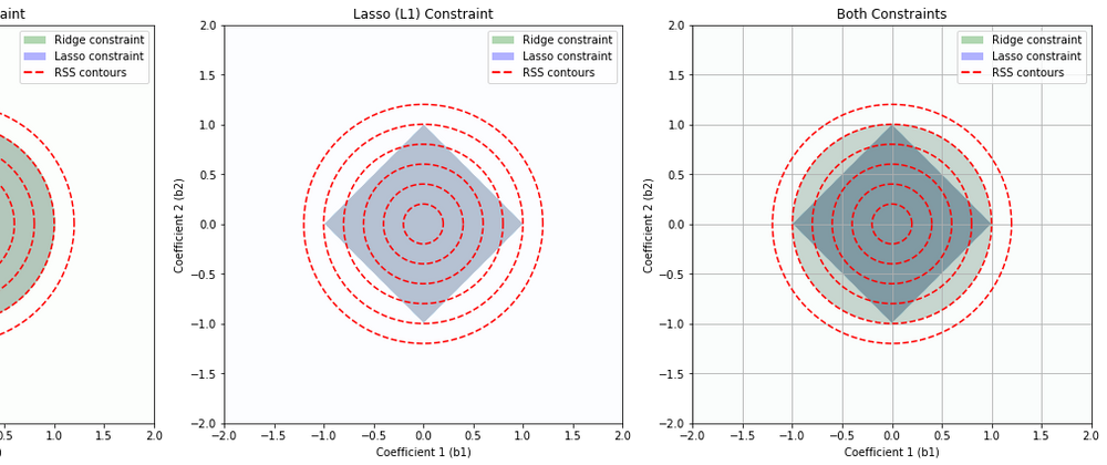
This set of diagrams shows how Ridge (L2) regularization and Lasso (L1) regularization impose different "constraint regions" on the values that the coefficients of a linear regression model can take.

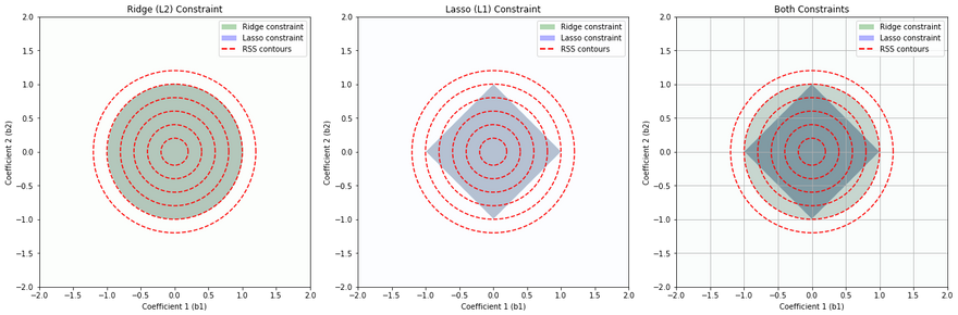
In each plot, the x and y axes represent the possible values of two coefficients in a linear regression model. For simplicity, we are considering a linear regression model with two coefficients, but this concept can be extended to more coefficients.

The colored regions (green for Ridge, blue for Lasso) show the sets of coefficient values that are allowed by the Ridge and Lasso constraints respectively, assuming a certain limit on the size of the coefficients. The limit is determined by the regularization parameter, which is not explicitly shown here.

The red dashed lines are contours of the Residual Sum of Squares (RSS), which is the quantity that linear regression tries to minimize. Each contour line represents a set of coefficient values that result in the same RSS.

• Ridge (L2) Constraint (Leftmost Plot): The Ridge constraint allows coefficient values that lie within a circle centered at the origin. This is because Ridge regularization penalizes the square of the coefficients, resulting in a circular region of allowable coefficient values. Ridge tends not to force coefficients to be exactly zero, so it typically does not produce sparse solutions.

• Lasso (L1) Constraint (Middle Plot): The Lasso constraint allows coefficient values that lie within a diamond centered at the origin. This is because Lasso regularization penalizes the absolute value of the coefficients, resulting in a diamond-shaped region of allowable coefficient values. The corners of the diamond are on the axes, which means Lasso can force some coefficients to be exactly zero when the optimal solution lies at a corner, leading to sparse solutions.

• Both Constraints (Rightmost Plot): This plot shows the constraints from both Ridge and Lasso regularization overlaid. The overlapped region shows the set of coefficient values that would be allowed by both Ridge and Lasso.

The points where the contours of the RSS intersect with the constraint regions represent the optimal solutions under each type of regularization. The optimal solution will be different for Ridge and Lasso due to the different shapes of their constraint regions.

Note: In real applications, you would typically use either Ridge or Lasso regularization, not both at the same time. This set of diagrams is meant to illustrate the differences between these two types of regularization.

Lasso Vs Ridge Vs Dropout in action

Lets take a simple example of real state data and use all three regression model to predict the outcome. I found this dataset Predicting House Prices. You can download this data and play with it.

To visualize and compare the predictions made by these models, you can create plots of the true values versus the predicted values. For a perfect model, all points would lie on a straight line (since the true value would always equal the predicted value). Deviations from this line show the errors in prediction. Here I created a simple python function to demonstrate this.

import pandas as pd
from sklearn.model_selection import train_test_split
from sklearn.linear_model import Lasso, Ridge
from sklearn.metrics import mean_squared_error
import tensorflow as tf

# load the data
df = pd.read_csv('data/kc_house_data.csv')

# drop 'id' and 'date' columns
df = df.drop(columns=['id', 'date'])

# split the data into features (X) and target (y)
X = df.drop('price', axis=1)
y = df['price']

# split data into training and test set
X_train, X_test, y_train, y_test = train_test_split(X, y, test_size=0.2, random_state=42)

# L1 (Lasso) regularization
lasso = Lasso(alpha=0.1)
lasso.fit(X_train, y_train)
y_pred = lasso.predict(X_test)
print(f'Lasso Mean Squared Error: {mean_squared_error(y_test, y_pred)}')

# L2 (Ridge) regularization
ridge = Ridge(alpha=0.1)
ridge.fit(X_train, y_train)
y_pred = ridge.predict(X_test)
print(f'Ridge Mean Squared Error: {mean_squared_error(y_test, y_pred)}')

# Neural Network with dropout
model = tf.keras.models.Sequential([
  tf.keras.layers.Dense(64, activation='relu', input_shape=(X_train.shape[1],)),  # input layer
  tf.keras.layers.Dropout(0.5),  # dropout layer
  tf.keras.layers.Dense(64, activation='relu'),  # hidden layer
  tf.keras.layers.Dropout(0.5),  # dropout layer
  tf.keras.layers.Dense(1)  # output layer
])

model.compile(optimizer='adam', loss='mean_squared_error')

model.fit(X_train, y_train, epochs=10, batch_size=32, validation_data=(X_test, y_test))


import matplotlib.pyplot as plt
import numpy as np

# Generate predictions
lasso_pred = lasso.predict(X_test)
ridge_pred = ridge.predict(X_test)
nn_pred = model.predict(X_test).flatten()  # flatten to convert from 2D to 1D array

# Create subplots
fig, axes = plt.subplots(1, 3, figsize=(15, 5))

# Lasso plot
axes[0].scatter(y_test, lasso_pred)
axes[0].plot([y_test.min(), y_test.max()], [y_test.min(), y_test.max()], 'k--', lw=3)
axes[0].set_title('Lasso: True vs Predicted')
axes[0].set_xlabel('True')
axes[0].set_ylabel('Predicted')

# Ridge plot
axes[1].scatter(y_test, ridge_pred)
axes[1].plot([y_test.min(), y_test.max()], [y_test.min(), y_test.max()], 'k--', lw=3)
axes[1].set_title('Ridge: True vs Predicted')
axes[1].set_xlabel('True')
axes[1].set_ylabel('Predicted')

# Neural Network plot
axes[2].scatter(y_test, nn_pred)
axes[2].plot([y_test.min(), y_test.max()], [y_test.min(), y_test.max()], 'k--', lw=3)
axes[2].set_title('Neural Network: True vs Predicted')
axes[2].set_xlabel('True')
axes[2].set_ylabel('Predicted')

plt.tight_layout()
plt.show()

Output:

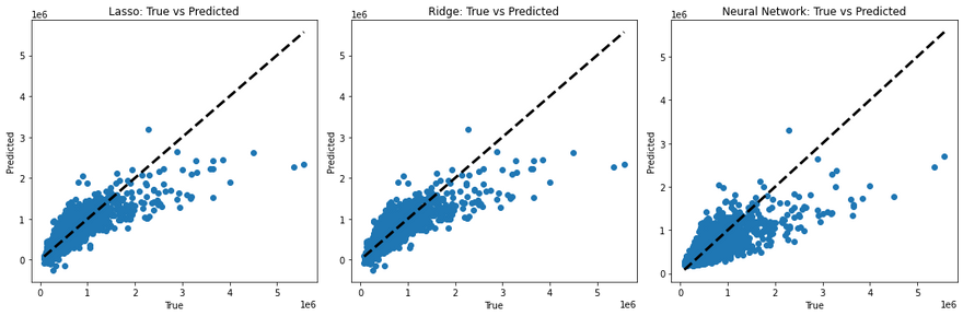
This code will generate a scatter plot for each model. The dotted line in each plot represents the ideal case where the true value equals the predicted value. The scatter points show the predicted values against the true values. If a model's predictions are perfect, all points should lie on this line. Therefore, the closer the points are to the line, the better the model's performance.